The Simplex Algorithm

1. The Simplex Algorithm LI Xiao-lei

2. preface • The two-variable LP program can be solved graphically. • Most real-life LPs have many variables. • In many industrial applications, the simplex algorithm is used to solve LPs with thousands of constraints and variables.

3. How to convert an LP to standard form • Before the simplex algorithm can be used to solve an LP, the LP must be converted into an equivalent problem in which all constraints are equations and all variables are nonnegative. An LP in this form is said to be in standard form.

4. EXAMPLE 1 • Leather limited manufactures two types of belts: the deluxe model and the regular model. Each type requires 1 sq yd of leather. A regular belt requires 1 hour of skilled labor, and a deluxe belt requires 2 hours. Each week, 40 sq yd of leather and 60 hours of skilled labor are available. Each regular belt contributes $3 to profit and each deluxe belt, $4.

5. EXAMPLE 1 • Define, X1=number of deluxe belts produced weekly X2=number of regular belts produced weekly • The LP is, Max z=4x1+3x2 (LP1) s.t. x1+ x2≤40 (Leather constraint) 2x1+ x2≤60 (Labor constraint) x1,x2≥0

6. Convert inequality constraints to equality constraints • Define for each ≤ constraint a slack variable si (si=slack variable for ith constraint). We define, s1=40- x1-x2 or x1+ x2+ s1=40 s2=60-2x1-x2 or 2x1+ x2 + s2=60 Note: a point satisfies the ith constraint if and only if si≥0.

7. LP1 in standard form Max z=4x1+3x2 (LP1’) s.t. x1+ x2 +S1 =40 2x1+ x2 +S2 =60 x1,x2,S1,S2≥0 Note: if constraint i of an LP is a ≤ constraint, we convert it to an equality constraint by addinga slack variable si to the ith constraint and adding the sign restriction si ≥0.

8. Similarly, to convert the ith ≥ constraint to an equality constraint, we define an excess variable (some times called a surplus variable) ei. Note: if the ith constraint of an LP is a ≥ constraint, it can be converted to an equality constraint by subtracting an excess variable ei from the ith constraint and adding the sign restriction ei≥0.

9. example Original LP, max z=20x1 + 15x2 s.t. x1≤100 x2≤100 50x1+ 35x2≤6000 20x1+ 15x2≥2000 x1,x2≥0

10. example Standard form LP, max z=20x1 + 15x2 s.t. x1 + s1=100 x2 +s2 =100 50x1+ 35x2 +s3 =6000 20x1+ 15x2 -e4=2000 xi≥0(i=1,2); s3≥0(i=1,2,3); e4≥0

11. Preview of the simplex algorithm • Suppose an LP with m constraints in standard form, max z= c1x1+ c2x2+…+ cnxn (1) s.t. a11x1+a12x2+…+a1nxn=b1 a21x1+a22x2+…+a2nxn=b2 … … am1x1+am2x2+…+amnxn=bm xi≥0(i=1,2,…,n)

12. We define, The constraints may be written as the system of equations Ax=b

13. Basic and nonbasic variables • Consider a system Ax=b of m linear equations in n variables (assume n≥m) • DEFINATION A basic solution to Ax=b is obtained by setting n-m variables equal to 0 and solving for the values of the remaining m variables. This assumes that setting the n-m variables equal to 0 yields unique values for the remaining m variables or, equivalently, the columns for the remaining m variables are linearly independent.

14. Basic and nonbasic variables • To find a basic solution to Ax=b, we choose a set of n-m variables (the nonbasic variables, or NBV) and set each of these variables equal to 0. Then solve for the values of the remaining n-(n-m)=m variables (the basic variables, or BV) that satisfy Ax=b.

15. Basic and nonbasic variables • The different choices of nonbasic variables will lead to different basic solutions. To illustrate, x1+x2 =3 -x2+x3=-1 We begin by choosing a set of 3-2=1 nonbasic variables. If NBV={x3} then BV={x1,x2}. We find that x1=2, x2=1, by setting x3=0. If NBV={x2} then we get x1=3, x2=0, x3=-1.

16. Basic and nonbasic variables • Some sets of m variables do not yield a basic solution. For example, x1+2x2+x3=1 2x1+4x2+x3=3 If we choose NBV={x3}, then x1+2x2=1 2x1+4x2=3 The system has no solution, there is no basic solution to BV={x1,x2}

17. Feasible solutions • DEFINATION Any basic solution to (1) in which all variables are nonnegative is a basic feasible solution(or bfs). THEOREM 1 The feasible region for any linear programming problem is a convex set. Also, if an LP has an optimal solution, there must be an extreme point of the feasible region that is optimal. THEOREM 2 For any LP, there is a unique extreme point of the LP’s feasible region corresponding to each basic feasible solution. Also, there is at least one bfs corresponding to each extreme point of the feasible region.

18. Feasible solutions Illustration of Leather Limited example, Max z=4x1+3x2 (LP1’) s.t. x1+ x2 +S1 =40 2x1+ x2 +S2 =60 x1,x2,S1,S2≥0

20. Adjacent basic feasible solutions • DEFINATION For any LP with m constraints, two basic feasible solutions are said to be adjacent if their sets of basic variables have m-1 basic variables in common.

21. How the simplex algorithm solves LPs in a max problem • Step1 find a bfs to the LP. We call this bfs the initial basic feasible solution. In general, the most recent bfs will be called the current bfs, so at the beginning of the problem the initial bfs is the current bfs. • Step2 determine if the current bfs is an optimal solution to the LP. If it is not, find an adjacent bfs that has a larger z-value. • Step3 Return to step2, using the new bfs as the current bfs.

22. How the simplex algorithm solves LPs in a max problem • If an LP in standard form has m constraints and n variables, there may be a basic solution for each choice of nonbasic variables. From n variables, a set of n-m nonbasic variables can be chosen in Different ways.

23. How the simplex algorithm solves LPs in a max problem • Thus, an LP can have at most basic solutions. • If we were proceed from the current bfs to a better bfs, we would surely find the optimal bfs after a finite number of calculations.

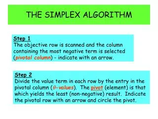
24. The Simplex Algorithm • Step1 convert the LP to standard form. • Step2 obtain a bfs (if possible) from the standard form. • Step3 determine whether the current bfs is optimal. • Step4 if the current bfs is not optimal, determine which nonbasic variable should become a basic variable and which basic variable should become a nonbasic variable to find a new bfs with a better objective function value. • Step5 use ero(elementary row operation)’s to find the new bfs with the better objective function value. Go back to step3.

25. example • The dakota furniture company manufactures desk, tables, and chairs. The manufacture of each type of furniture requires lumber and two types of skilled labor: finishing and carpentry. 48 board feet of lumber, 20 finishing hours, and 8 carpentry hours are available. A desk sells for $60, a table for $30, and a chair for $20. demand for desks and chairs is unlimited, but at most five table can be sold. Dakota wants to maximize total revenue.

26. example • Defining the decision variable as x1=number of desks produced x2=number of tables produced x3=number of chairs produced • Dakota is the following LP: max z=60x1+30x2+ 20x3 s.t. 8x1+ 6x2+ x3≤48 (lumber constraint) 4x1+ 2x2+1.5x3≤20 (finishing constraint) 2x1+1.5x2+0.5x3≤8 (carpentry constraint) x2 ≤5 (limitation on table demand) x1,x2,x3≥0

27. example • Convert the LP to standard form max z=60x1+30x2+ 20x3 s.t. 8x1+ 6x2+ x3 +s1 =48 4x1+ 2x2+1.5x3 +s2 =20 2x1+1.5x2+0.5x3 +s3 =8 x2 +s4=5 x1,x2,x3,s1 ,s2,s3 ,s4≥0 Note: the row 0 for the objective function is z -60x1-30x2-20x3=0

28. example • Putting rows 1-4 together with row 0 and the sign restrictions yields the equations and basic variables. Canonical form 0

29. example • The feasible solution for the initial canonical form has BV={s1,s2,s3,s4} ={0,48,20,8,5} and NBV={x1,x2,x3}={0,0,0} The feasible solution, z=0,s1=48,s2=20,s3=8,s4=5,x1=x2=x3=0 Note: a slack variable can be used as a basic variable for an equation if the right-hand side of the constraint is nonnegative.

30. example • Is the current basic feasible solution optimal? To determine whether there is any way that z can be increased by increasing some nonbasic variables at their current values of zero. Note: from z=60x1+30x2+ 20x3 we can observe that x1 has the most negative coefficient in row 0. we call x1 the entering variable.

31. example • Determine the entering variable We choose the entering variable (in a max problem) to be the nonbasic variable with the most negative coefficient in row 0(ties may be broken in an arbitrary fashion). Increasing x1 may cause a basic variable to become negative.

32. example • How to increasing x1( holding x2=x3=0) ? From row 1 s1≥0 for x1≤48/8=6 From row 2 s2≥0 for x1≤20/4=5 From row 3 s3≥0 for x1≤8/2=4 From row 4 s4≥0 for all values of x1 Note: to keep all the basic variables nonnegative, the largest that we can make x1 is min{48/8,20/4,8/2}=4. Also for any row in which the entering variable had a positive coefficient, the row’s basic variable became negative when the entering variable exceeded right-hand side of row coefficient of entering variable in row (10)

33. example • How to increasing x1( holding x2=x3=0) ? The ratio test When entering a variable into the basis, compute the ratio in (10) for every constraint in which the entering variable has a positive coefficient. The constraint with the smallest ratio is called the winner of the ratio test. The smallest ratio is the largest value of the entering variable that will keep all the current basic variables nonnegative.

34. example • Find a new basic feasible solution: pivot in the entering variable In which row does the entering variable become basic? Always make the entering variable a basic variable in a row that wins the ratio test. In example, to make x1 a basic variable in row 3, we use elementary row operations to make x1 have a coefficient of 1 in row 3 and a coefficient of 0 in all other rows. This procedure is called pivoting on row 3; and row 3 is the pivot row. The final result is that x1 replaces s3 as the basic variable for row 3. The term in the pivot row that involves the entering basic variable is called the pivot term.

35. example • To make x1 a basic variable in row 3 by performing the following ero’s. ero 1 create a coefficient of 1 for x1 in row 3 by multiplying row 3 by ½. The resulting row is x1+0.75x2+0.25x3+0.5s3=4 (row 3’) ero 2 to create a zero coefficient for x1 in row 0, replace row 0 with 60(row 3’) +row 0. z+15x2-5x3+30s3=240 (row 0’) ero 3 to create a zero coefficient for x1 in row 1, replace row 1 with -8(row 3’)+row 1. -x3+s1-4s3=16 (row 1’) ero 4 to create a zero coefficient for x1 in row 2, replace row 2 with -4(row 3’)+row 2. -x2+0.5x3+s2-2s3=4 (row 2’)

36. example • x1 does not appear in row 4. we don’t need to perform an ero to eliminate x1 from row 4. Canonical form 1

37. example • The feasible solution for the canonical form 1 has BV={z,s1,s2,x1,s4} and NBV={s3,x2,x3} The feasible solution, z=240,s1=16,s2=4,x1=4,s4=5,x2=x3=s3=0 In obtaining canonical form 1 from the initial canonical form, we have gone from one bfs to a better (larger z-value) bfs. Note: the initial bfs and the improved bfs are adjacent. The procedure used to go from one bfs to a better adjacent bfs is called an iteration (or sometimes, a pivot) of the simplex algorithm.

38. example • Try to find a bfs that has a still larger z-value. Rearranging row 0’ to solve for z, z=240-15x2+5x3-30s3 • Increasing x2 by 1 will decrease z by 15. • Increasing s3 by 1 will decrease z by 30. • Increasing x3 by 1 will increase z by 5. Thus we choose to enter x3 into the basis. Note: the rule for determining the entering variable is to choose the variable with the most negative coefficient in the current row 0. since x3 is the only variable with a negative coefficient in row 0’, it should be entered into the basis.

39. example • To determine how large x3 can be. • From row 1’: s1=16+x3 all values of x3 • From row 2’: s2=4-0.5x3 x3≤4/0.5=8 • From row 3’: x1=4-0.25x3 x3≤4/0.25=16 • From row 4’: s4=5 all values of x3 The largest we can make x3 is min{4/0.5,4/0.25}=8

40. example • To determine how large x3 can be. Also can be discovered by using (10) and the ratio test: Row 1’: no ratio (x3 has negative coefficient in row) Row 2’:4/0.5=8 Row 3’:4/0.25=16 Row 4’:no ratio (x3 has a nonpositive coefficient in row 4) Thus, the smallest ratio occurs in row 2’, and row 2’ wins the ratio test.

41. example • Use ero’s to make x3 a basic variable ero 1 create a coefficient of 1 for x3 in row 2’ by replacing row 2’ with 2(row 2’) -2x2+x3+2s2-4s3=8 (row 2’’) ero 2 to create a zero coefficient for x3 in row 0’, replace row 0 with 5(row 2’’) +row 0’. z+5x2+10x2+10s3=280 (row 0’’) ero 3 to create a zero coefficient for x3 in row 1’, replace row 1’ with row 2’’+row 1’. -2x2+s1+2s2-8s3=24 (row 1’’) ero 4 to create a zero coefficient for x3 in row 3’, replace row 3’ with -1/4(row 2’’)+row 3’. x1+1.25x2-0.5s2+1.5s3=2 (row 3’’)

42. example • x3 already has a zero coefficient in row 4’. we don’t need to perform an ero to eliminate x3 from row 4’. Canonical form 2

43. example • From canonical form 2, we find BV={z,s1,x3,x1,s4} and NBV={s2,s3,x2} It yields the following bfs: z=280,s1=24,x3=8,x1=2,s4=5,s2=s3=x2=0 Since the bfs’s for canonical forms 1 and 2 have 4-1=3 basic variables in common (s1,s4,x1), they are adjacent basic feasible solutions. Now the second iteration (or pivot) has been completed.

44. example • If we rearrange row 0’’ and solve for z, we obtain z=280-5x2-10s2-10s3 We see that increasing any nonbasic variable will cause z to decrease. this might lead us to believe that our current bfs is an optimal solution. • Is a canonical form optimal(max problem)? A canonical form is optimal( for a max problem) if each nonbasic variable has a nonnegative coefficient in the canonocal form’s row 0.

45. Summary of the simplex algorithm for a max problem • Step 1 convert the LP to standard form. • Step 2 find a basic feasible solution. • Step 3 if all nonbasic variables have nonnegative coefficients in row 0, the current bfs is optimal. If any variables in row 0 have negative coefficients, choose the variable with the most negative coefficient in row 0 to enter the basis. We call this variable the entering variable.

46. Summary of the simplex algorithm for a max problem • Step4 use ero’s to make the entering variable the basic variable in any row that wins the ratio test. After the ero’s have been used to create a new canonical form, return to step 3, using the current canonical form.

47. Representing simplex tableaus • Rather than writing each variable in every constraint, we often used a shorthand display called a simplex tableau. • For example, z+3x1+x2=6 x1+s1=4 2x1+x2+s2=3

48. Representing simplex tableaus • This format makes it very easy to spot basic variable: Just look for columns having a single entry of 1 and all other entries equal to 0 (s1 and s2). In our use of simplex tableaus, we will encircle the pivot term and denote the winner of the ratio test by *.

49. Using the simplex algorithm to solve minimization problems • There are two different ways that the simplex algorithm can be used to solve minimization problems. • We illustrate these methods by solving the following LP: min z=2x1-3x2 s.t. x1+ x2≤4 x1- x2≤6 (LP2) x1,x2≥0

50. Method 1 • We can find the optimal solution to LP 2 by solving LP 2’: max -z=-2x1+3x2 s.t. x1+ x2≤4 x1- x2≤6 (LP2’) x1,x2≥0 Initial tableau: The ratio test indicates that x2 should enter the basis in row 1.