The simplex algorithm
The simplex algorithm. The simplex algorithm is the classical method for solving linear programs. Its running time is not polynomial in the worst case. It does yield insight into linear programs, however, and is often remarkably fast in practice.

The simplex algorithm
E N D
Presentation Transcript
The simplex algorithm • The simplex algorithm is the classical method for solving linear programs. • Its running time is not polynomial in the worst case. • It does yield insight into linear programs, however, and is often remarkably fast in practice. • The simplex algorithm bears some similarity to Gaussian elimination (iteration)
Gaussian elimination begins with a system of linear equalities whose solution is unknown. • In each iteration, we rewrite this system in a equivalent form that has some additional structure. • After some number of iterations, we have rewritten the system so that the solution is simple to obtain.
To find the solution of the following system of linear equations: 2x + y - z = 8 ----- (1) -3x - y - 2z = -11 ----- (2) -2x + y + 2z = -3 ----- (3) Eliminate x in both (2) and (3): (2) + 3/2(1) (2) 0x + 1/2 y + 1/2 z = 1 ----(2) (3) + (1) (3) 0x + 2 y + z = 5 ----(3)
Eliminate y in (3): (3) - 4 (2) (3) 0x + 0y – z = 1 -----(3) We have that (upper triangle) 2x + y – z = 8 ----(1) 0x + 1/2 y + 1/2 z = 1 ----(2) 0x + 0y – z = 1 ----(3) Then, we have z = -1 from (3), y = 3 from (2) and z=-1, and x = 2 from (1) and y=3,z=-1
An example of the simplex algorithm Subject to We first convert the linear program from standard form into slackform.
Convert standard form to slack form • Non-negative constraints are the only inequality constraints. • All other constraints are equality constraints • Introduce slack variables x4 , x5 ,x6 for inequality X4 = 30 – x1 – x2 – 3x3 X5 = 24 – 2x1 – 2x2 – 5x3 X6 = 36 – 4x1 – x2 – 2x3
Clearly, slack variables x4 , x5 ,x6 must be non-negative, and they are called basic variables, and the original variables x1 , x2 ,x3 are called non-basic variables. Therefore, we have x1 , x2 ,x3 , x4 , x5 ,x6 >= 0 2. Let the object function be in slack form. z = 0 + 2x1 – 3x2 + 3x3
A solution is feasible if all of x1, x2, ..., x6 are Nonnegative • there can be an infinite number of feasible solutions since there are 6 variables and only 3 equations • Eq-2
Any setting of variables x1 , x2 ,x3 will define values for x4 , x5 ,x6 . • A solution isfeasibleif all x1 , x2 ,x3 , x4 , x5 ,x6 are non-negative • Basic solution is obtained by setting all non-basic variables to zero and then calculating the values for basic variables as well as the value of object function z. • (x1 , x2 ,x3 , x4 , x5 ,x6, z) = (0,0,0,30,24,36,0).
thebasic solution: set all the (non-basic) variables on the right-hand side to 0and then compute the values of the (basic) variables on the left-hand side. • is the basic solution • it has value z = (3 · 0) + (1 · 0) + (2 ·0) = 0. • If a basic solution is also feasible, we call it a basic feasible solution. • If a basic solution is not feasible, we shall call Initialize-simplex procedure to find a basic solution if it exists.
Our goal, in each iteration, is to reformulate the linear program so that the basic solution has a greater objective value. 1.We choose a non-basic variable with positive coefficient in objective function. 2. We increase the value of this variable to a limit that will violate any of these constraints. 3. Then the non-basic variable as entering variable and the basic variable as leaving variable in this constraint will exchange places. This is pivoting.
increasing the value of x1. As we increase x1, the values of x4, x5, and x6 all decrease. • we cannot allow any of them to become negative in order to be a feasible solution. • The third constraint is the tightest constraint, and it limits how much we can increase x1 (=9). • Obtain a new constraint from 3rd constraint
To rewrite the other constraints with x6 on the right-hand side, we substitute x6 for x1 • we obtain • X4= • X5= 6 – 3/2 X2 - 4 X3 + 1/2 X6
Similarly, to rewrite our linear program in the following form: • Eq3. • this operation is called a pivot. • a pivot chooses a non-basic variable xe (x1 ),called the entering variable, and a basic variable xl (x6) called the leaving variable, and exchanges their roles.
The linear program described in eq-3 is equivalent to the linear program described in eq-2. • However the values of object function z are different. If we set zero to non-basic variables and calculate the values for basic variables and finally find the value for z, we have (9, 0, 0, 21, 6, 0) and z = (3*9) + (1*0) + (2*0) = 27.
we wish to find a new variable whose value might be increased. • We do not increase x6 since its coefficient is negative so this will decrease z • We can tryx2 or x3 , say x3. • The third constraint is again the tightest one, and we will therefore rewrite the third constraint so that x3 is on the left-hand side and x5 is on the right-hand side. We then substitute this new equation into eq-3 and obtain the new, but equivalent, system
Eq-4 • We obtain (33/4, 0, 3/2, 69/4, 0, 0) and z= 111/4. (27.75) The only way to increase the value of z is to increase x2. since it is positive term.
We increase x2to 4, and it becomes non-basic. • we solve eq-4 for x2and substitute in the other equations to obtain Eq-5.
At this point, all coefficients in the objective function are negative. As we shall see later in this chapter, this situation occurs only when we have rewritten the linear program so that the basic solution is an optimal solution. • for this problem, the solution (8, 4, 0, 18, 0, 0), with objective value 28, is optimal.
Check the slack variables in the original form with the final solution for x1 , x2 ,x3 = 8, 4, 0, we have that x4 , x5 ,x6 = 18, 0, 0. That is, only slack variable x4has big slack. • The values of coefficients in the original form of the example are integers, however in many real problems, it is real numbers. The coefficients intermediate form and the solution may also be real numbers.
Pivoting • We now formalize the procedure for pivoting. • The procedure PIVOT takes as input a slack form, given by the tuple (N, B, A, b, c, v), the index l of the leaving variable xl , and the index e of the entering variable xe. It returns the tuple describing the new slack form.
PIVOT works as follows. • Lines 2–5 compute the coefficients in the new equation for xebyrewriting the equation that has xlon the left-hand side to instead have xeon the left-hand side. • Lines 7–11 update the remaining equations by substituting the right-hand side of this new equation for each occurrence of xe.
Lines 13–16 do the same substitution for the objectivefunction, and • lines 18 and 19 update the sets of non-basic and basic variables. • Line 20 returns the new slack form. As given, if ale = 0, PIVOT would cause an error by dividing by 0, • PIVOT is called only when ale ≠ 0.
Lemma 29.1: Consider a call to PIVOT(N, B, A, b, c, v, l, e) in which ale ≠ 0. Let the values returned fromthe call be , and let denote the basic solution after the call. Then
The formal simplex algorithm • we could have had several other issues to address: • How do we determine if a linear program is feasible? • What do we do if the linear program is feasible, but the initial basic solution is not feasible? • How do we determine if a linear program is unbounded? • How do we choose the entering and leaving variables?
We therefore assume that we have a procedure INITIALIZE-SIMPLEX(A, b, c) that takes as input a linear program instandard form, that is, an m × n matrix A = (aij), an m-dimensionalvector b = (bi), andan n-dimensionalvector c = (cj). • If the problem is infeasible, it returns a message that the programis infeasible and then terminates. Otherwise, it returns a slack form for which the initial basic solution is feasible.
Lemma for L has a feasible solution • Let L be a linear program in standard form, .
Let Lmaxbe the following linear program with n+1 variables. maximize –x0 subject to Sumj=1 to n aij xj - x0 <= bi for i=1,…, m xj >= 0 for j=0,…,n. Then, L is feasible iff the optimal objective solution for Lmaxis 0.
The procedure SIMPLEX takes as input a linear program in standard form, as just described. It returns an n-vector that is an optimal solution to the linear program.
Convert a general form to standard form • If the objective function to be minimize, then negative the coefficients of the objective function to obtain the maximize form. • If a variable xi has a negative constraint replace occurrences of xi with x’I - x’’I, and add constraints: x’I >= 0 and x’’I >= 0 . • If a constraint is in equality form, then replace it with two inequality forms: ‘>= ‘ and ‘<=‘ • If a constraint is a ‘>=‘ form, then multiply the constraint by -1 to obtain a ‘<=‘ form.
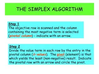
The SIMPLEX procedure works as follows. In line 1, it calls the procedure INITIALIZESIMPLEX(A, b, c), described above, which either determines that the linear program isinfeasible or returns a slack form for which the basic solution is feasible. The main part of the algorithm is given in the while loop in lines 2–11. If all the coefficients in the objective function are negative, then the while loop terminates. Otherwise, in line 3, we select a variable xewhose coefficient in the objective function is positive to be the entering variable.
While we have the freedom to choose any such variable as the entering variable, we assume that we use some prespecified deterministic rule.
Next, in lines 4–8, we check each constraint, and we pick the one that most severely limits the amount by which we can increase xe without violating any of the non-negativity constraints. • the basic variable associated with this constraint is xl . Again, we may have the freedom to choose one of several variables as theleaving variable, but we assume that we use some pre-specified deterministic rule.
If none of the constraints limits the amount by which the entering variable can increase, the algorithm returns "unbounded" in line 10. Otherwise, line 11 exchanges the roles of the entering and leaving variables by calling the subroutine PIVOT(N, B, A, b, c, v, l, e), as described above.
Lines 12–15 compute a solution for the original linear-programming variables by setting all the nonbasic variables to 0 and each basic variable to bi . • We shall see that this solution can be proven to be an optimal solution to the linear program. • Finally, line 16 returns the computed values of these original linear-programming variables.
To show that SIMPLEX is correct, we first show that if SIMPLEX has an initial feasible solution and eventually terminates, then it either returns a feasible solution or determines that the linear program is unbounded. Then, we show that SIMPLEX terminates. Finally, we can show that the solution returned is optimal.
Lemma 29.2: Given a linear program (A, b, c), suppose that the call to INITIALIZE-SIMPLEX in line 1 ofSIMPLEX returns a slack form for which the basic solution is feasible. Then if SIMPLEX returns a solution in line 16, that solution is a feasible solution to the linear program. If SIMPLEX returns "unbounded" in line 10, the linear program is unbounded.
At each iteration, SIMPLEX maintains A, b, c, and v in addition to the sets N and B. Althoughexplicitly maintaining A, b, c, and v is essential for the efficient implementation of the simplex algorithm, it is not strictly necessary. • In other words, the slack form is uniquely determined by the sets of basic and nonbasic variables. Before proving this fact, we prove a useful algebraic lemma.
Lemma 29.3: Let I be a set of indices. For each i Є I, let αiand βibe real numbers, and let xibe a real-valued variable. Let γ be any real number. Suppose that for any settings of the xi, we have Then αi = βifor each i Є I, and γ = 0.
Lemma 29.4: Let (A, b, c) be a linear program in standard form. Given a set B of basic variables, theassociated slack form is uniquely determined. • it is possible that an iteration leaves the objective value unchanged. This phenomenon is called degeneracy
The objective value is changed by the assignment in line 13 of PIVOT. • Since SIMPLEX calls PIVOT only when ce > 0, the only way for the objective value to remainunchanged (i.e., )is for to be 0. This value is assigned as in line 2 of PIVOT. • Since we always call PIVOT with ale ≠ 0, we see that for to equal 0, and hence the objectivevalue to be unchanged, we must have bl = 0.
Indeed, this situation can occur. Consider the linear program • Suppose that we choose x1 as the entering variable and x4 as the leaving variable. After pivoting, we obtain
At this point, our only choice is to pivot with x3 entering and x5 leaving. Since b5 = 0, the objective value of 8 remains unchanged after pivoting: • The objective value has not changed, but our representation has.
We say that SIMPLEX cycles if the slack forms at two different iterations are identical, in which case, since SIMPLEX is a deterministic algorithm, it will cycle through the same series of slack forms forever. • Lemma 29.5: If SIMPLEX fails to terminate in at most iterations, then it cycles.
Cycling is theoretically possible, but extremely rare. • It is avoidable by choosing the entering and leaving variables somewhat more carefully. • One option is to perturb the input slightly so that it is impossible to have two solutions with the same objective value. • A second is to break ties lexicographically, and a third is to break ties by always choosing the variable with the smallest index. The last strategy is known as Bland's rule.
Lemma 29.6: If in lines 3 and 8 of SIMPLEX, ties are always broken by choosing the variable with the smallest index, then SIMPLEX must terminate. • Lemma 29.7: Assuming that INITIALIZE-SIMPLEX returns a slack form for which the basic solution is feasible, SIMPLEX either reports that a linear program is unbounded, or it terminates with a feasible solution in at most iterations.

