Download
1 / 87
870 likes | 1.19k Vues
Application of Transport Optimization Codes to Groundwater Pump and Treat Systems. Internet Training Seminar September 24, 2003. Today’s Presenters. Dave Becker U.S. Army Corps of Engineers Hazardous, Toxic and Radioactive Waste Center of Expertise ( dave.J.becker@usace.army.mil )

E N D
Application of Transport Optimization Codes to Groundwater Pump and Treat Systems Internet Training Seminar September 24, 2003
Today’s Presenters • Dave Becker • U.S. Army Corps of Engineers Hazardous, Toxic and Radioactive Waste Center of Expertise (dave.J.becker@usace.army.mil) • Karla Harre • Naval Facilities Engineering Service Center (karla.harre@navy.mil) • Dr. Barbara Minsker • University of Illinois (minsker@uiuc.edu) • Rob Greenwald • GeoTrans, Inc. (rgreenwald@geotransinc.com) • Dr. Chunmiao Zheng • University of Alabama (czheng@wgs.geo.ua.edu) • Dr. Richard Peralta • Utah State University (richard.peralta@usurf.usu.edu)
Remedial OptimizationFor P&T Systems • Remediation System Evaluation (RSE) or Remedial Process Optimization (RPO) provides a broad assessment of… • Goals and exit strategy • Below-ground performance • Above-ground performance • Monitoring and reporting • Potential for alternate technologies • Pumpage optimization is a subset or a component of these more general optimization evaluations • Trying to determine the “best” extraction/injection strategy assuming P&T is the most appropriate technology
Presentation Outline • What is “transport optimization”? • Why perform transport optimization? • General optimization process • Formulating problems • Solving problems • Recent DOD “ESTCP” groundwater remediation optimization study • Project Background • Example: Umatilla • Example: Blaine • Lessons Learned • Further Information
What is “Transport Optimization”? • Optimization algorithms coupled with existing groundwater flow and transport models that determine an “optimal” set of pumping/injection well rates & locations wells PLUME Regional Flow Source Area Extraction well Injection well Example: Minimize total pumping rate subject to: - TCE < 5 ppb at each cell within current plume extent after 5 yr. - TCE < 1 ppb at each cell outside current plume extent (all times) - extraction volume equals injection volume
Why Perform Transport Optimization? • “Hydraulic Optimization” can be too limiting for many sites (1999 EPA Demonstration project) • Optimization based only on ground water FLOW model • Focus is on containment, cannot optimize based on concentration or cleanup times Hydraulic Optimization
Hydraulic Optimization wells Plume Regional Flow Extraction well Injection well Inward flow constraint Example: Minimize total pumping rate subject to: - inward flow at plume boundary = plume containment - extraction volume equals injection volume
Why Perform Transport Optimization? • “Hydraulic Optimization” can be too limiting for many sites (1999 EPA Demonstration project) • Optimization based only on ground water FLOW model • Focus is on containment, cannot optimize based on concentration or cleanup times • Transport Optimization • Optimization based on ground water FLOW and TRANSPORT model • Not just containment…considers concentrations and cleanup times
Why Perform Transport Optimization? • Assuming a model is being used to evaluate pumping alternatives…the optimization algorithms will yield improved strategies relative to strategies determined by trial & error model simulations • Potential benefits of improved strategies include • Faster cleanup • Lower life-cycle cost
General Optimization Process • Start with a real-life problem for which you are seeking the “best” or “optimal” solution • Formulate the Problem. Develop an “optimization formulation” that describes the essential elements of the real world problem in mathematical terms to establish… • The parameters for which optimal values are to be determined • The criteria for determining that one solution is better than another • The rules for allowing some solutions and disallowing others • Solve the Problem. Select and apply an appropriate methodology to search possible and allowable combinations of pumping strategies for an “optimal” solution
Formulation Components (Terminology) • Decision Variables • What we are determining optimal values for • Objective Function • The mathematical equation being minimized or maximized • Value can be computed once the value of each decision variable is specified • Serves as the basis for comparing one solution to another • Constraints • Limits on values of the decision variables, or limits on other values that can be calculated once the value of each decision variable is specified
Formulation Components Example Max x2+y2 Subject to: -4 y 4 -2 x 2 2x + 3y 12 Objective Function Decision Variables Constraints
Example of Formulation Process for a Real-Life Situation • Real-Life Problem • What is the optimal driving route between home to work? Office One-way Home
Example of Formulation Process for a Real-Life Situation • Formulation must establish… • The decision variables • Combinations of roads/turns between my house and work • The objective function (some possibilities) • Minimize distance traveled • Minimize travel time • Minimize number of traffic lights • The constraints (some examples) • Must travel on paved roads • No more than four traffic lights allowed • Cannot go wrong way on a one-way street
Mathematical Descriptions are Often Difficult… • Example: Minimize Travel Time • How do you mathematically account for traffic when calculating time of travel for a selected route of travel? • How do you estimate speed on the interstate? • Does it depend on time of day? • Does it depend on day of the week? • Simplifications are invariably required in the formulation process • Many alternative formulations are generally possible, each may have a different optimal solution
Solve the Formulation • Global optimization algorithms use “heuristic” approaches to find the highest peak or lowest valley • Genetic algorithm • Simulated annealing • Tabu search • Artificial neural network Peaks and Valleys “Heuristic” refers to methods that work based on “rules of thumb” but there is no specific mathematical proof that it does work and no guarantee of optimality
Real-World Problem: Peaks and Valleys Highest Peak Lowest Valley
Optimization Process:Ground Water Remediation Problems • Preliminary Tasks • Understand site-specific goals and constraints • Verify/update flow & transport model until it is considered valid for design purposes • Obtain detailed information required to develop the formulations • State formulation(s) in mathematical terms • Objective function • Constraints • Select optimization codes/algorithms & solve formulations • Revise formulations and solve as needed
Types of Information Collected:Ground Water Remediation Problems • Cost components • One-time “capital” costs (now or in the future) • Annual costs • Point of exposure, point of compliance Schematic
Point of Exposure and Point of Compliance Point of Exposure must have concentrations below a specified limit to protect receptors at or near this location Property Boundary Point of Compliance must have concentrations below a specified limit to protect potential receptors downgradient Plume Extraction wells Regional Flow
Types of Information Collected:Ground Water Remediation Problems • Cost components • One-time “capital” costs (now or in the future) • Annual costs • Point of exposure, point of compliance • Containment zones Schematic
Containment Zone Schematic Containment Zone Regional Flow Plume Containment Zone defined to prevent the plume from spreading
Types of Information Collected:Ground Water Remediation Problems • Cost components • One-time “capital” costs (now or in the future) • Annual costs • Point of exposure, point of compliance • Containment zones • Cleanup criteria and time period • System capacity • Pumping/injection limits • Drawdown/water level limits Schematic
Water Level Limit Private Well Land Surface Lowest water level allowed to protect private well Well Screen
Types of Information Collected:Ground Water Remediation Problems • Cost components • One-time “capital” costs (now or in the future) • Annual costs • Point of exposure, point of compliance • Containment zones • Cleanup criteria and time period • System capacity • Pumping/injection limits • Drawdown/water level limits • Limit on capital cost, etc. • Other planned actions (such as source removal) that may impact future remedy performance
Formulation Components:Ground Water Remediation Problems • Decision Variables • Locations of extraction/injection wells • Rates at each extraction/injection well over time • Potential objective functions (select only one unless using a multi-objective algorithm) • Total life-cycle cost {minimize} • Cleanup time {minimize} • Contaminant mass remaining in aquifer {minimize} • Contaminant mass removed from aquifer {maximize} • Potential constraints (as many as you want…here are some examples) • Limits on pumping rates at specific wells or total pumping rate • Limits on concentrations (at specific locations/times) • Restrictions on well locations • Limits on aquifer drawdown at specific locations • Financial constraints such as limits on capital costs
Optimization Codes:Ground Water Remediation Problems • Dr. Chunmiao Zheng (University of Alabama), Modular Groundwater Optimizer (MGO) • Genetic algorithms • Simulated annealing • Tabu search • Dr. Richard Peralta (Utah State Univeristy), Simulation Optimization Modeling Systems (SOMOS) • Genetic algorithms • Simulated annealing • Tabu search • Genetic algorithms coupled with artificial neural network
Modular Groundwater Optimizer (MGO) • Simulation Components • MODFLOW for groundwater flow • MT3DMS for multi-species contaminant transport • Optimization Components • Global optimization (heuristic search) techniques • Genetic algorithms (GA) • Simulated annealing (SA) • Tabu search (TS) • Integrated techniques • Global optimization techniques + response functions for greater computational efficiency
MGO: Setup of Optimization Modeling • Input files for MODFLOW (no modification) • Input files for MT3DMS (no modification) • An optimization input file specifying • Optimization Solver (GA, SA, TS) • Output options • Decision variables (flow rates, well locations) • Objective function • Constraints
MGO: Additional Information • Code Compatibility • MODFLOW • MT3DMS • Platforms that incorporates MGO • Groundwater Vistas
Copyright August 2003 Simulation / Optimization Modeling System (SOMOS) • Optimization Software for Managing: • Groundwater Flow • Solute Transport • Conjunctive Use • SOMOS is easy-to-use Windows-based S/O modeling software • SOMOS has a comprehensive set of heavy-duty optimizers to most efficiently address the spectrum of management optimization problems • SOMOS significantly improves planning and management and can help optimally manage water resources systems of unlimited size • SOMOS results from twenty years experience developing optimization models and applying them to real-world problems, including 11 pump-and-treat (PAT) systems and many large and small scale water supply problems • SOMOS has detailed documentation, tutorials, and error checking Developed by: Systems Simulation /Optimization Laboratory Department of Biological and Irrigation Engineering Utah State University, Logan, UT 84322 – 4105 Contact: richard.peralta@usurf.usu.edu
Applications SOMOS handles large and complex problems and has been applied to many real-world problems. Some examples are: • Minimizing cost of TCE plume containment at Norton AFB: • Optimization yielded 23% cost reduction from base strategy • System was built, strategy was implemented and successful • TCE contaminant plume management: Minimizing TCE mass remaining at Massachusetts Military Reservation, CS-10 plume, while preventing plume expansion • Optimization yielded 6% improvement from base strategy, at less cost • Constructed system is operating successfully • Cache Valley sustained yield optimization problem: Maximizing sustained yield of stream-aquifer system • Optimal strategy showed sustainable pumping could increase 40% • causing management change • Applications performed at three sites for this ESTCP project For more applications: http://www.usurf.org/units/wdl
SOMOS Features • Windows-based SOMOS runs in background, while user employs other programs. • SOMOS’ spread-sheet based pre-processor, SOMOIN, simplifies input file preparation (availability depends on version). • SOMOS’ professional design has detailed input error-checking and error messages. • Buttons on SOMOS’ user-friendly interface speed accessing/editing I/O files, and optimizations. • SOMOS’ flexibility allows run restarts, result merges, stepwise, sequential, and simultaneous optimization, full control over constraints and bounds in time and space. • SOMOS’ automation allows considering multitudinous candidate wells in a run and speeds sequential running of multiple optimization actions. • SOMOS includes a 2-D spreadsheet-based tool for mapping layered aquifer parameters, well locations and hypothetical capture zones (availability depends on version). • SOMOS is being included within groundwater modeling packages such as Visual MODFLOW and Groundwater Vistas
SOMOS Features (vary with version) • Applicability:Any confined or unconfined aquifer system that can be modeled. • Simulators: MODFLOW, MT3DMS, SEAWAT, Response Matrix, Response Surface, Artificial Neural Networks, Others. • 12 Optimizers: Including Simplex, Gradient Search, Branch & Bound, Outer Approximation, Genetic Algorithm (GA) linked with Tabu Search (GA-TS) and Simulated Annealing (SA) linked with Tabu Search (SA-TS). • Optimization Problem Types: linear, quadratic, nonlinear, mixed integer, mixed integer nonlinear, multi-objective, stochastic (i.e. under uncertainty). • Controllable Variables: ground-water pumping, gradient, cell-head, head at well casing; surface water diversion, flow, & head; aquifer/surface body seepage; contaminant concentration, mass remaining & removal; user-definable variables. • Management Goals:Can optimize for 90+ distinct objective functions plus user-defined objective and multi-objective optimization.
ESTCP Demonstration Project • Goal of project • Demonstrate application of “transport optimization” at real world sites • Evaluate the benefits and costs of using optimization algorithms versus the traditional trial-and-error modeling approach • Make transport optimization technology more accessible • Training • Code availability
Project Setup • “Transport optimization” applied at 3 sites • Umatilla Chemical Depot, Oregon • Tooele Army Depot, Utah • Former Blaine Naval Ammunition Depot, Nebraska • At each site, three different optimization formulations were developed • Each formulation was solved (over a fixed time period) by… • two groups applying the coupled simulation-optimization approach • one group running the contaminant transport model using trial-&-error (to serve as a scientific control) • Use of two groups provided greater confidence in results, a comparison of code performance, and more insight into the “beyond the code” efforts required to solve the problems
Project Team • ESTCP and EPA provided funding, USACE also provided support • Diverse project management team • NFESC - Karla Harre, Laura Yeh • EPA-TIO - Kathy Yager • USACE - Dave Becker • GeoTrans, Inc. - Rob Greenwald, Yan Zhang • University of Illinois - Dr. Barbara Minsker • Transport optimization modelers • Utah State University - Dr. Richard Peralta (SOMOS) • University of Alabama - Dr. Chunmiao Zheng (MGO)
Demonstration Sites * TCE simulated is combined plume of TCE, PCE, TCA, DCE, and RDX
Formulation Process For Each Site • Perform site visit and review site data • Understand the real-life situation • Explore real-life objectives and constraints with the installations • Initial discussion of how to convert real life situation into mathematical description • Review site groundwater flow and transport model • Receive assurance from installation that they consider the model predictions acceptable for use for remediation design purposes • Important because the transport model provides the mathematical relationship between the decision variable values (the pumping locations/rates) and terms in the constraints/objective function
Formulation Process For Each Site • Develop 3 “optimization formulations” based on further interaction with the installations • Select an “objective function” to be minimized (or maximized) • Specify a set of constraints to be satisfied • Worked with installation to establish final mathematical representations of key problem components, such as… • Cost coefficients (e.g., cost of new well, cost to treat each gpm, etc.) • Nature of the relationships between the decision variables and other terms in the objective function and/or constraints (e.g., is the cost to treat each gpm constant, or does it change based on flow rate and/or contaminant concentrations?)
Optimization Formulations POE = Point of Exposure; POC = Point of Compliance
Example: Umatilla • Goal: cleanup 2 constituents • RDX: 2.1 ug/L • TNT: 2.8 ug/L • Current system • System capacity: 2 GAC units @ 1300 gpm • 3 extraction wells • 3 infiltration basins • Expect cleanup in 17 years Site Location Current System & Plume Distribution
CURRENT SYSTEM IF1 IFL EW-3 EW-1 EW-4 Treatment Plant IF2 IF3
Umatilla Objective Function:Formulation 1 • Minimize Total Cost Until Cleanup Total Cost = CCW + CCB + CCG + FCL + FCE + VCE + VCG + VCS • CCW: Capital Costs of new Wells • CCB: Capital Costs of new Recharge Basins • CCG: Capital Costs of new GAC units • FCL: Fixed Costs of Labor • FCE: Fixed Costs of Electricity • VCE: Variable Costs of Electricity • VCG: Variable Costs of changing GAC units • VCS: Variable Costs of Samplingfuture costs are discounted to yield Net Present Value
Umatilla: Cost Terms • Up-Front costs • New well and piping: $75K • Put EW-2 in service: $25K • New recharge basin: $25K • New GAC unit (325 gpm): $150K • Fixed Annual Costs (each year until cleanup) • Labor (fixed): $237K/yr • Electric (fixed): $3.6k/yr • Variable Costs Depending on Solution (complicated) • Electric based on pump rate at specific wells • GAC changeout based on influent concentration • Sampling costs due to plume area Details: Variable Electric Costs