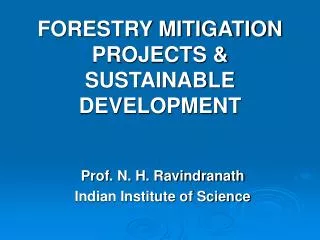
Methodological Issues in Forestry Mitigation Projects
Methodological Issues in Forestry Mitigation Projects. Ken Andrasko Office of Atmospheric Programs U.S. Environmental Protection Agency, Washington, DC, USA Jayant Sathaye, LBNL at Workshop on Climate Change Mitigation Forestry Projects in India, Bangalore, July 10-12, 2003.

Methodological Issues in Forestry Mitigation Projects
E N D
Presentation Transcript
Methodological Issues in Forestry Mitigation Projects Ken Andrasko Office of Atmospheric Programs U.S. Environmental Protection Agency, Washington, DC, USA Jayant Sathaye, LBNL at Workshop on Climate Change Mitigation Forestry Projects in India, Bangalore, July 10-12, 2003
I. Project Experience • Projects -- IPCC Special Report LULUCF, 2000 • “Planned set of activities that are • confined to one or more geographic locations in the same country • belong to specified time periods and institutional frameworks, and • allow monitoring and verification of greenhouse gas (GHG) emissions or changes in carbon stock” • Much experience with LULUCF projects, but the number for which GHG elements have been explicitly evaluated is limited: c. 20-30
GHG Project Experience • About 3.5 million ha of land in about 30 projects in 19 countries being implemented during the 1990s • For 21 projects w/ sufficient data available: • Estimated accumulated carbon uptake over the project lifetime in 11 forestation projects on 0.65 Mha amounts to about 30 Mt C, • Estimated accumulated emissions avoided in 10 forest protection and management over the project lifetime on 2.86 Mha amounts to between 46 to 53 Mt C • Several issues may affect these estimates.
Example: Reforestation - Forest Restoration • Brazil - Atlantic Forest Projects • Since 1999, purchased over 20,000 ha of lands now managed for Asian water buffalo • Project = improved buffalo management, reforestation & natural regeneration w/ native species, agroforestry. • Land is owned and managed by Brazilian NGO Sociedade de Pesquisa em Vida Selvagem (SPVS) • Total cost = $17 million, about 7.5 million tons of CO2 over 30 years • 3 separate projects funded by American Electric Power, General Motors, Texaco Credit: Bill Stanley, TNC
Kyoto process: Sinks inclusion in Art. 3.3, 3.4 (Annex I) & CDM (non-Annex I) limited by inadequate experience & methods to address sinks technical issues • LULUCF projects share most issues with energy projects -- except duration of benefits (permanence). • Perception: adequate methods & data exist for A, R, D in Annex I. • Perception: CDM sinks in non-Annex I difficult to measure & high leakage. So: A & R; no forest protection • Key technical issues: • baseline setting by activity and location • additionality of activities (envir. & financial) • leakage of GHG benefits offsite • duration (permanence) of LUCF benefits. • Envir. & sus. dev. (eg, avoid incentives for planting monocultures).
II. Project Concepts:Estimating Baseline and GHG BenefitPrior to project implementation
Project Concepts: Monitoring GHG BenefitDuring Project Implementation Note: P (measured and adjusted for leakage) can be above P (estimated); Monitored GHG benefit would then be less than the estimated amount
Evolving Steps for Estimating Baseline and Project GHG Reductions: WRI/WBCSD draft 7/03 1. Identify project and its primary GHG effect 2. Check project eligibility 3. Undertake preliminary evaluation of secondary effects - Leakage and life-cycle effects 4. Check if project is “surplus” (additional) to regulation
Evolving Steps Baseline and Project: 2 6. Select an approach and set a baseline for each primary effect: - Project-specific, or GHG performance standard baseline 7. Identify and assess relevance of secondary effects 8. Calculate project emissions reductions 9. Classify emissions reductions into direct and indirect: ( Under control of the developer or not).
II. Methods for Setting Baselines, & Examples from Case Studies • Project-specific • Baselines are set specific to each project • Concern: Project baselines set strategically to maximize credits • Multi-project Baselines or Emissions Factors • Generic baselines may reduce transaction costs, be transparent, and provide consistency across projects • Setting minimum performance benchmarks would avoid rewarding projects with poor practices • Fixed vs. Adjustable Baselines • Fixed baseline would reduce uncertainty • Adjustable baselines would ensure more realistic offsets, but would increase cost and uncertainty • Periodic adjustments may be one solution
Examples of Project Baseline Scenarios Credit: Bill Stanley, TNC
Methods matter: Comparison of 5 baseline-setting approaches: Rio Bravo project, Belize(Draft: Winrock Intertl-EPA analysis, in prep.) Source: Brown et al. 2002, Winrock International analysis
Baseline Steps: Identify spatial and temporal boundaries for baseline, &project. • Step 1: Determine Baseline Afforestation, Reforestation, or Other LU Rates • Assess land-use trends and changes in C stocks for candidate area and activities • Step 2: Determine Likely Locations of Future Af/Reforestation, Deforestation, etc. • Identify 2-5 key baseline drivers • Assess historical trends and projection into future • Step 3: Estimate Net Emissions or Sequestration for Each Unit of Baseline Deforestation/Reforestation
Baseline: Quantify probability of current land use changing without project
Additionality: Can determine relative additionality of proposed project activities • Land transformation matrices can project probability of future land change without project. • Method steers developers & regulators towards areas and activities with high likelihood of being additional. • Method reflects heterogeneity of land uses, & avoids binary, yes/no additionality.
Baseline Driver Example:% Land-Use Change, Forest to Non-forest: 1975-96. Chiapas, Mexico.Factors: Distance from Roads, by Population Density Roads, by Population 0 -1000 m 1000 - 2000 m > 2000 m 0 hab/km2 43 25 7 >0 a 15 55 38 24 >15 a 30 67 50 34 >30 hab/km2 78 62 42 Source: ECOSUR, & de Jong et al., 2000
Vegetation cover in 1975, Chiapas, Mexico from Remote Sensing data Source: ECOSUR, Chiapas, Mexico; & de Jong et al, 2002.
Vegetation cover in 1996, Chiapas, Mexico: rate rate of land cover and use change Source: ECOSUR, Chiapas, Mexico; & de Jong et al, 2002.
Carbon emissions from land use change, 1975 - 1996 Total emission 119, 465,774 tC Source: ECOSUR, Chiapas, Mexico; & de Jong et al, 2002.
Predicted Deforestation: Noel Kempff Project, Bolivia -- GIS model projections Deforestation projection, 2000 - 2040 Baseline drivers = nearness to road & ag croplands; population changes Source: Bill Stanley, TNC from GEOMOD by M. Hall, 2002
1992 1986 Project-Scale Land Use Analysis for Baseline: Jambi, Indonesia: 1986-92 Rizaldi et al, 2003:
PredictedLand Use: 1992 Real Land Use: 1992 Figure 6. Comparison between real and predicted land use/cover of Jambi province and Batanghari district using the logit regression equations. Rizaldie et al, 2003
Jambi Case: Mitigation Scenario Results, and Effect of Adjusting Baseline. Rizaldi et al, 2003
Example: EPA Mississippi Case: Testing 4 coarse to fine resolution data approaches to Baseline Setting & Additionality • Green: national forests • Brown: marginal croplands,, flooded every 2 yrs. • Project: restore wetland hardwood species • 4 counties
Mississippi Case Study: Test 4 different baseline-setting approaches • Can generic or ‘multi-project’ baselines be established that could apply to any project within a large region? • Or, are county-level or sub-county baseline needed to capture land-use dynamics at project scale? • What are the tradeoffs between cost and accuracy when moving from coarse (county-level) to fine (pixel-level GIS) methods? • Can existing national data sources be used to allow for transferable methods across the U.S.?
Mississippi case: Approach & Findings • Baseline: county-level land-use change using national NRI data: all cropland has same baseline rate afforestn. • If add 2-3 baseline drivers (frequency of cropland flooding, crop type), have 5-7 baseline rates. • if use remote sensing/GIS, have dozens of baseline rates. But: requires ground truthing; data issues. • Allows “relative additionality” if baseline varies by category. Vs. single, binary yes/no additionality. • Leakage: Testing bottom-up approach by land category, & comparing with US national ag/forest FASOM model default values for activity shifting & market leakage. • Permanence: comparing insurance and discounting
Project Concepts: Adjusting Baseline and GHG BenefitAfter some years of project implementation Baseline valid for 5-10 years? Influenced by policy? Note: B (adjusted) can be below B (estimated) -- Adjusted GHG benefit would then be less than monitored amount
III. Methods for Estimating Leakage • Definitions • Examples from different approaches • Philippines, Indonesia, Mexico, US • Which approaches to use in India? Discussion?
Leakage = Unintended Change in GHG Flux Outside the Boundaries of Project, as Result of Project Activities • Types: 1) Activity shifting, 2) market leakage (from changes in traded products) • Assess likelihood of leakage for project activities & location: Decision trees help identify land & product markets affected, & activity shifting. • Option 1: Avoid via Project Design or Location: • Project components supply fiber/ land demanded • Option 2: Estimate Leakage, & Include in GHG accounting • Use top-down models, default values, or bottom-up estimates from project
Leakage Example: Mississippi, US, Case: • Brown lands = Project: marginal cropland into afforestration. • If retire cropland, but new cropland cleared outside project, = activity shifting. • If afforestation produces wood products traded on market, = market effect.
Bottom-Up Leakage Decision Tree for Deforestation Projects in Tropics Source: Aukland, Moura Costa, Brown 2002
Jambi Case: Effect of considering Leakage in Mitigation Scenarios. Rizaldi et al, 2003
Chiapas, Mexico Leakage Study: Bottom- Up Approach on Farmer Small Holdings • Plan Vivo: farmer-made drawing of his baseline & project land use (c. 1-5 ha). • Survey instrument: questions re Plan Vivo intended vs. actual land use & adjacent plots. • Survey: technicians visit 10% of 450 farmers, and 3 community Plan vivo projects. • Questions identify specific types of leakage: activity shifting; market (wood products). • Hypothesis: minimal leakage. In progress.
Leakage: Top-Down Modeling Approach: EPA Work w/ National Ag/Forest Economic Model May Allow Projects to Target Low-Magnitude Regions in U.S. Preliminary leakage estimates for large regional programs, using FASOM national-scale model Afforestation Program Leakage Results, as % Northeast 23 Lake States 18 Corn Belt 30 Southeast 40 South-central 42 Avoided Deforestation Leakage Results, as % No Harvesting Harvesting Allowed Pacific Northwest-east side 8 7 Northeast 43 41 Lake States 92 73 Corn Belt 31 –4 South-central 28 21 Source: Murray, McCarl, Lee 2002
IV. Permanence: Adjust GHG accounting for duration, saturation, other factors • Duration: reversibility of carbon storage. • Options: Use insurance, take discounts, use project portfolios to spread risk. • Saturation: biological limit to carbon storage. • Saturation may reduce value of forestry and ag offsets relative to permanent emission offsets. • 1 - 49% discount forestry options for U.S.. (50 yr.) • 45 - 62% for ag soil options for U.S. (saturate: 20 yrs.) Source: McCarl et al. 2001 in press
DRAFT EPA Framework for Project Guidance Step 1. Feasibility screening Step 2. Establish and apply baseline Coarse-scale baseline credible? Identify project activity and region NO Use fine-scale, sub-county baseline method YES Passes institutional, regulatory additionality? Baseline-adjusted project GHG benefits viable? NO NO YES YES Step 3. Final adjustments, monitor, verify, report Estimate project GHG benefits (unadjusted) • Other adjustments • if necessary • leakage (default, specific) • duration Review leakage defaults HIGH Adjusted project GHG benefits remain viable? Monitor, verify, report final, adjusted GHG project benefits YES LOW NO
Measuring Changes in Carbon Stocks of Forestry Projects • Carbon pools -- Live and dead biomass, soil, and wood products • Techniques and tools exist to measure carbon stocks in project areas relatively precisely depending on the carbon pool • Monitoring cost between $1-5 per hectare and US$0.10-0.50 per t C have been reported by a few projects
Carbon Measurement Needs by Project Type Red: needs to be measured; Gree: recommended Yellow may be necessary Brown et al, 2000
Associated Impacts and Sustainable Development • Site-specific experience exists documenting the socioeconomic and environmental impacts of LULUCF projects • Critical factors that affect contributions of LULUCF projects to sustainable development include: • Extent and effectiveness of local community participation • Transfer and adoption of technology • Capacity to develop and implement guidelines and procedures • Addressing factors can alleviate project permanence • Biodiversity not yet assessed
Issue 5: Can We Identify Co-Benefits and Co-Effects of Mitigation Options, and Design Policies to Promote them?Case study: Lower Mississippi River Basin: Water Quality Changes due to Sequestration Activities • Initial analysis by RTI/Texas A&M for EPA on water quality implications of sequestration activities. • Delta states show largest water quality improvement per unit GHG reduced. • Significant (~9%) reductions in N loadings entering Gulf at $25 & $50/tC incentive prices. Source: Pattanayak et al. 2002
Ideal case study to explore approaches to project issues • Data richness and availability • GIS images at fine resolution • Large enough scale to test ‘spatial approach’ (e.g., low 1,000s of ha) • Key baseline drivers that affect land-use change and management well known (incl. policies) • Area includes croplands and forest lands • Targets area where options look promising: ability to quantify issues & generate co-benefits