TOPICS TO BE DISCUSSED
300 likes | 502 Vues
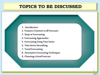
1. Introduction 2. Features Common to all Forecasts 3. Steps in Forecasting 4. Forecasting Approaches 5. Forecasting Using Time Series 6. Time Series Smoothing 7. Trend Forecasting 8. Associative Forecasting Techniques 9. Choosing a Good Forecast. TOPICS TO BE DISCUSSED.

TOPICS TO BE DISCUSSED
E N D
Presentation Transcript
1.Introduction 2. Features Common to all Forecasts 3. Steps in Forecasting 4. Forecasting Approaches 5. Forecasting Using Time Series 6. Time Series Smoothing 7. Trend Forecasting 8. Associative Forecasting Techniques 9. Choosing a Good Forecast TOPICS TO BE DISCUSSED
Introduction • What is a Forecast? • A guess or estimation of future events based on previous experience. • How does your area of study use forecasts? • How does an Operations Manager use a forecast? • Help managers design a system • Help managers plan a use for the system • Used for Capacity Planning, Sales, Manpower, & Inventory • Forecasting is Both Long Term and Short Term. • Strategic, Tactical and Operational • Forecasting is not an Exact Science. • Based on Experience, Judgment, Technical Expertise, & Luck • Generally Forecasting is Done on Many Levels. • Product Demand is forecasted by Marketing or Sales • Manpower and Equipment needs are forecasted by Operations • Monetary Needs is forecasted by Finance
Make or Buy Facility Definition Resource Planning Aggregate Plan Forecasting Rough Cut Capacity Planning Master Production Schedule MRP Detailed Capacity Planning Shop Floor Control Purchasing How Forecasting Fits in Production Cycle
Features Common to All Forecasts • Assumes that the same underlying causes that existed in the past will be present • in the future. • Forecasts are rarely perfect. • Group Forecasts tend to be more accurate as forecasting errors among groups • usually have a canceling effect. • Accuracy decreases as the time period increases. If Forecasts are not perfect then why should we spend time and money on developing them?
Steps in Forecasting • 1. Determine the Purpose of the Forecast and When it will be needed. • Level of Detail • Level of Accuracy • Budget constraints • Intended use • 2. Establish a Time Horizon that the forecast must cover. • The longer the less accurate • Sufficient amount of data • 3. Select the Forecast Technique. • Depends on accuracy • Experience • Time Span • Cost • 4. Gather and Analyze the appropriate Data & Prepare the Forecast. • 5. Monitor the Forecast Performance • If not performing then modify the technique, data, and/or requirements.
ForecastingApproaches • Qualitative vs Quantitative • Qualitative Forecasting is very subjective. • Based on judgment, opinion, consumer surveys, Delphi & sales people. • Use when: • Conditions are changing - Time is short - Obsolete Data • Consumer surveys get Buyer’s feedback, if handled correctly • To act as a sanity check for quantitative results • Quantitative approach is based on historical or associative models. • Quantitative models are based on some abstract mathematical model to describe • future events. • Time Series Analysis is a historical method • It tries to uncover a pattern or cycle in the empirical data relative to time. • Also tries to remove any random and nonrandom errors. • Associative Method attempts to predict the future based on the relationship • between two variables. • The variable that is being predicted is dependent on the value of the known • variable. Delphi
Forecasting Using Time Series Data • Time Series is a time ordered sequence of observations taken at regular intervals • over a period of time. • Future values of a series are predicated on the assumption that past information is • repeatable. • The forecaster must determine if a pattern exists and what is the cycle of the pattern. • These patterns might be classified in terms of: • Trends: long term upward or downward movement of data • Seasonal: short term regular variations • Cycles: longer term variations • Irregular Variations: Unpredictable random variations. • A demand forecast should be based on the time series of past demand rather than • sales. • Differentiate between demand and sales • Previous sales may not have kept up with demand
Time Based Smoothing • Naïve Forecasts • Use last period’s actual results for this period’s forecast. • Benefits: Easy of use; Low Costs; Easy to understand; Quick • Disadvantages: Questionable accuracy • Is the increased accuracy warrant the extra time and cost of another method? • Moving Average • Uses a number of the most recent actual data values in generating a forecast. • MAn = (Di)/n • i = “age” of the data • n = number of periods in the moving average • D = Actual Demand with the age i • MA3 would imply a three period moving average • The more period used the less accurate • Doesn’t reflect the current environment • Slower to respond to changes • Each data point is weighted the same • Advantage • Easy to compute • Easy to Understand • Disadvantage • Accuracy • Responsiveness to changes
Time Based Smoothing (con’t) • Weighted Moving Average • Addresses one of the disadvantages of not being responsive to change • associated with the Simple Moving Average. • Applies a weighted factor to each of the periods used in the averaging. • The more recent periods are weighted more heavily. • MAn = (WDi) • w is the weight of the period demand D: {0<w< 1} • An issue is how to define the a value for the weighting factor. • Exponential Smoothing • Each new forecast is based on the previous forecast plus a percentage of the difference • between the previous forecast and the actual value of the previous period. • New Forecast = Old Forecast + (percentage of error)(Actual - Old Forecast) • Ft= Ft-1+ ( D t-1 - F t-1 ) • 0 << 1 ; Commonly values between .05 and .5 are used. • The closer it’s value to zero the slower the forecast will be adjust to forecast errors • Selecting the smoothing constant is basically a matter of trial and error. • Take the average of the first four values average • value will change until forecasting error is minimal • Impact of the error of a single period is ; (1- ) t-1
Time Based Smoothing (con’t) • Strengths of Exponential Smoothing • Easy to use especially on a large number of short term forecasts. • Emphasis is placed on recent data • Little skilled labor requirements to upkeep • Can Incorporate trend and seasonal components • Weaknesses of Exponential Smoothing • Not appropriate for small data collection requiring accuracy • Not based on statistical model building methods • Arbitrary of initial smoothing constants • Relationship to Moving Average • Moving average is based on N number of data points. (i.e.N= 3 for 3 month MA) • Exponential smoothing will be impacted by all previous data points, with the impact • diminishing with age. • The comparison of influence of the MA to the Exponential Smoothing is found by calculating α. • α= 2/(N+1) • So a 3 month moving average would have an α = 2/(3+1) = 0.5
Trend Forecasting • Techniques for Trend • The trend component of a time series reflects the effects of any long term factors • on the series. • Linear Trend • Plot data and transcribe a line through the data points (graphical). • Develop a Linear Trend Equation • Yt = a + bt • Y is the forecast for period t • t is the number of time periods • a is the value of Y when t=0 • b is the slope of the line • Once you have determined the equation of the line then you can predict any • future point by changing t. • Equations: • b = n (t*y) - t y • n t2 - ( t)2 • a = y - b t • n
Associative Forecasting Techniques • Associative Techniques rely on identification of relayed variables that can be used to predict values of the variable of interest. • The predictor variable is called the Independent variable. • The variable being predicted is called the Dependent variable. • Linear Regressions use describes the linear relationships between two variable. • There are a number of methods for defining the linear regression equation. The most common is the Least Squares method. • Yc = a + bx • Yc = Dependent variable • x = Independent variable • b = slope of line • a = Y value when x = 0 • Notice the similarity to the Linear Time series • Equations: • b = n (x*y) - x y a = y - b x • n x2 - ( x)2 n • Multiple Linear Regressions use multiple Independent variables to predict the Dependent variable.
Associative Forecasting Techniques (con’t) • There are several measures to determine how well an Independent variable can predict a Dependent variable. • Standard Error of the Estimate (SEE) • Measures the mean square vertical deviations of the actual observations from the • fitted regression line. • Provides bounds within which the true value will fall. (Standard Deviation) • Correlation Coefficient (r) can define the strength and direction of the relationship. • The range is between -1.00 and +1.00 • A -1.00 says that there is a one to one relationship but that they move in opposite • directions. • A +1.00 says that there is a one to one relationship and they move in the same • direction. • A 0.00 says there is no relationship. • A value of -1.00 is just as valuable as a +1.00 • Coefficient of Determination (R2)indicates the percentage of total variation explained by the regression line.
Accuracy of Forecast • Monitor for erratic demand, look for outliers • Is forecasting method effectively tracking demand • Which parameters (N & alpha) provides best accuracy • Allow for safety stock • Two Measures of Forecast Accuracy: • MAD (Mean Average Deviation) MAD = | Actual – Forecast| n MSE ( Mean Squared Error) MSE = ( Actual – Forecast) 2 n-1 MSE will highlight outliers more so than MAD. USE MAD and MSE for Selection of appropriate forecast.
Controlling the Forecast A forecast is appropriate when the errors exhibit only random variations. If the forecast exhibits a non random error then it needs to be reevaluated. Forecasts can be monitored by either Tracking Signals or Control Charts Tracking Signal Tracking Signal = ( Actual – Forecast) MAD Focus is on evaluating cumulative error MAD is updated using Exponential smoothing MAD t = MAD t-1 + ( |Actual – Forecast| t – MAD t-1 ) MAD1= | Actual – Forecast| / n Tracking Signal results are compared to predetermined limits . Based on judgment and experience
Controlling the Forecast • Control Charts • Evaluated of validity is based on error being within a upper and lower control limits. • Monitors individual error • Assumptions of methods: • Forecast errors are randomly distributed around a mean of zero. • The distribution of errors is normal. • Control limits are defined as a predetermined number of standard deviations from the mean. • The square root of the MSE is used as the standard deviations. UCL = 0 + z (MSE) ½ LCL = 0 - z (MSE) ½ • Use when: • Mean is equal to zero • There is no trend in error • Error can be described by a normal distribution
Choosing A Good Forecast • No one technique works best in every situation. • The two most important factors are: Cost & Accuracy • Best Forecast is not necessarily the most accurate; It is the most Cost Effective one • . • Other Relevant Factors • Availability of data • Experience with different types of forecasting models • Time allotment • Forecast horizon • Moving Averages & Exponential Smoothing are Short Term in nature; • Trend Equations tend to be more Long Term • Use more than one technique for comparison • Never accept a Quantitative result without doing a sanity check. • Elements of a Good Forecast • Timely • Sufficient Accuracy • Reliable • In Writing • Simple to Understand & use • Meaningful units to the decision maker
Delphi Approach Delphi approach is based on obtaining various expert opinions. If the estimates are widely varied the information is shared and the experts are asked to resubmit a new estimate. The assumption is that the experts will modify their estimates towards the mean. Demand 1st estimate 2nd estimate 3rd estimate Dual result
( y) ( t) b= Linear Trend y Value Rise ( y) Y- Intercept (a) Run ( t) Time (t)
Linear Trend y yi y0 yi yi yi Value yi yi yi yi yi yi yi Time (t)
Moving Average Demand (D) 42 40 43 40 41 39 46 44 45 38 40 Moving Average n = 3 months MA3= 42+40+43 /3 = 41.66 = 40+43+40 /3 = 41.0 = 43+40+41 /3 = 41.33 = 40+41+39 /3 = 40.0 = 41+39+46 /3 = 42.0 = 39+46+44 /3 = 43.0 = 46+44+45 /3 = 45.0 = 44+45+38 /3 = 42.33 = 45+38+40 /3 = 41.0 Period (t) 1 2 3 4 5 6 7 8 9 10 11 Assumes: each period has a .333 weighting
Weighted Moving Average Period (t) 1 2 3 4 5 6 7 8 9 10 11 Demand (D) 42 40 43 40 41 39 46 44 45 38 40 Weighted Moving Average Let: t-1 = 50%; t-2 = 30%; t-3 = 20% MA3 = (.2)42+(.3)40+(.5)43 = 41.9 = (.2)40+(.3)43+(.5)40 = 40.9 = (.2)43+(.3)40+(.5)41 = 41.1 = (.2)40+(.3)41+(.5)39 = 39.8 = (.2)41+(.3)39+(.5)46 = 42.9 = (.2)39+(.3)46+(.5)44 = 43.6 = (.2)46+(.3)44+(.5)45 = 44.9 = (.2)44+(.3)45+(.5)38 = 41.3 = (.2)45+(.3)38+(.5)40 = 40.4
Naïve Approach Period (t) 1 2 3 4 5 6 7 8 9 10 11 12 Demand (D) 42 40 43 40 41 39 46 44 45 38 40 Forecast (F) 42 40 43 40 41 39 46 44 45 38 40
Exponential Smoothing • Ft = Ft-1 + (D t-1 - F t-1 ) Period (t) 1 2 3 4 5 6 7 8 9 10 11 Demand (D) 42 40 43 40 41 39 46 44 45 38 40 Forecast (F0.2)Forecast (F0.9) 45 45 44.4 42.3 43.5 40.2 43.4 42.7 42.7 40.3 42.4 40.9 41.7 39.2 42.6 45.3 42.9 44.1 43.3 44.9 42.2 38.7 41.8 39.9 Let F0= 45 = .2 F2 = 45 + .2 (42 - 45) = 44.4 F8 = 41.7 + .2 (46 - 41.7) = 42.6 F3 = 44.4 + .2 (40 - 44.4) = 43.5 F9 = 42.6 + .2 (44 - 42.6) = 42.9 F4 = 43.5 + .2 (43 - 43.5) = 43.4 F5 = 43.4 + .2 (40 - 43.4) = 42.7 F10 = 42.9 + .2 (45 - 42.9) = 43.3 F6 = 42.7 + .2 (41 - 42.7) = 42.4 F11 = 43.3 + .2 (38 - 43.3) = 42.2 F7 = 42.4 + .2 (39 - 42.4) = 41.7 F12 = 42.2 + .2 (40 - 42.2) = 41.8
Linear Trend Period (t) 1 2 3 4 5 6 7 8 9 10 11 66 Demand (D) 42 40 43 40 41 39 46 44 45 38 40 458 t*y t2 Forecast 42 1 41.59 80 4 41.6 129 9 41.61 160 16 41.62 205 25 41.63 234 36 41.64 322 49 41.65 405 81 41.66 380 100 41.67 440121 41.68 2749 506 Yt = a + b*t Yt = 41.58 + .0091*t • b = n (x*y) - x y = (11)(2749) - (66)(458) = .0091 • n x2 - ( x)2 11(506) - (66)2 • a = y - b x = (458) - .0091(66) = 41.58 • n 11
SEE = (Yi - Y)2 n-2 Example 4: SEE 2 SEE 1 SEE 2 SEE 1 SEE
+3.75 -3.75 Tracking Signal Time
UCL = 0 + z (MSE) ½LCL = 0 - z (MSE) ½ UCL LCL Control Chart 0 Time
