Download
1 / 65
650 likes | 865 Vues
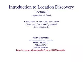
Introduction to Location Discovery Lecture 9 September 29, 2005 EENG 460a / CPSC 436 / ENAS 960 Networked Embedded Systems & Sensor Networks. Andreas Savvides andreas.savvides@yale.edu Office: AKW 212 Tel 432-1275 Course Website http://www.eng.yale.edu/enalab/courses/2005f/eeng460a.

E N D
Introduction to Location Discovery Lecture 9 September 29, 2005EENG 460a / CPSC 436 / ENAS 960 Networked Embedded Systems &Sensor Networks Andreas Savvides andreas.savvides@yale.edu Office: AKW 212 Tel 432-1275 Course Website http://www.eng.yale.edu/enalab/courses/2005f/eeng460a
Lecture Outline • Ecolocation • Probabilistic localization methods • Camera Based Localization • Rigidity • Other topics mentioned in discussion • Robust Quatrilaterals • Robustness and secure localization • Radio Interferometric localization
Radio Signal Strength: Ecolocation (Yetvali et. al USC & Bosch) • Initiation: • Node with unknown location (Unknown Node) initiates localization process by broadcasting a localization packet. • Nodes at known reference locations (Reference Nodes) collect RSS readings and forward them to a single point. • Procedure: • Determine the ordered sequence of reference nodes by ranking them on collected RSS readings. The ordering imposes constraints on the location of the unknown node. • For each location grid-point in the location space determine relative ordering of reference nodes and compare it with RSS ordering to determine how many of the ordering constraints are satisfied. • Pick the location that maximizes the number of satisfied constraints. If there is more than one such location, take their centroid.
“Constraints” & “Sequences” A 1 B B 2 4 C C 3 3 A 4 D 2 1 D E E B:1 C:2 D:3 E:4 R1 R2<R1 R3<R2 R4<R3 R3<R1 R4<R3 R4<R1 • Reference nodes (B,C,D,E) ranked into ordered sequenceby RSS readings. • The sequence of reference nodes changes with the location of the unknown node (A). Ideal Scenario: DAB < DAC => RB > RC Constraint on the location of the unknown node. RSS relationships between all reference nodes forms the constraint set.
Error Controlling Localization Real World Scenario: Multipath fading introduces errors in RSS readings which in turn introduce errors in the constraint set. Location estimate accuracy depends on the percentage of erroneous constraints. • The inherent redundancy in the constraint set helps withstand errors due to multi-path effects. • Analogous to error control coding. • Error Controlling Localization:Ecolocation Constraint construction inherently holds true for random variations in RSS measurements up to a tolerance level of |Ri - Rj|.
Ecolocation Examples No Erroneous Constraints 14% Erroneous Constraints A: Reference Node P: True Location of unknown node E: Ecolocation Estimated Location 22% Erroneous Constraints 47% Erroneous Constraints
Simulations Simulation Parameters Compared with four other localization techniques – Proximity Localization, Centroid, MLE, Approximate Point in Triangle (APIT). • RF Channel Parameters • Path loss exponent (η) • Standard deviation of log-normal shadowing model (σ) • Node Deployment Parameters • Number of reference nodes (α) • Reference node density (β) • Scanning resolution (γ) • Random placement of nodes Averaged over 100 random trials with 10 random seeds.
Simulation Results Da: Average inter reference node distance
Systems Implementation • Outdoors: • Represents a class ofobstruction free RF channels. • Eleven MICA 2 motes placed randomly on the ground in a 144 sq. m area in a parking lot. Locations of all motes are estimated and compared with true locations. • All motes in radio range and line of sight of each other. • Indoors: • Represents a class ofobstructive RF channels. • Twelve MICA 2 motes (Reference nodes) are placed randomly on the ground in a 120 sq. m area in an office building. • A MICA 2 mote (Unknown node) is placed in five different locations to be estimated. • All motes in radio range but only a subset in line of sight of each other.
Systems Implementation Results Locations estimated using Ecolocation, MLE and Proximity methods. Results suggest a hybrid localization technique.
Conclusion and Future Work Conclusion: • Ecolocation performs better than other RF based localization techniques over a range of RF channel conditions and node deployment parameters. • Simulation and experimental results suggest that a Hybrid Localization technique may provide the bestaccuracy. Future Work: • Exploring Hybrid Localization technique further. • Making Ecolocation more efficient using greedy search, multi-resolution search algorithms. • Analytical background for Ecolocation. • Measuring localization costs (Time, Throughput, Energy) for various realistic system designs and protocols.
Bayesian Filtering For Location Estimation(Fox et. al [Fox02]) • State estimators - probabilistically estimate a dynamic system’s state from noisy observations • In system theory, the information that dynamic system model gives us about the system is called system state • A system model is a set of equations that describe the system state. • The variables in the system model are the state variables
Bayesian Filters • In localization, state is the location of an entity • State representation is based on noisy sensor measurements • In simple cases, state can be just position in 2D • In more complex cases, state can be a complex vector including position in 3D, linear and rotational velocities, pitch, roll, yaw, etc.
Bayesian Filters • State (location) at time t is represented by random variable(s) x(t). • At each time moment, Bayesian filter represents a probability distribution over x(t) called belief • If we assume a sequence of time indexed sensor observations the belief becomes This is the probability distribution over all possible locations (states) x at time moment t, based on all possible sensor data available at time moment t (earlier and present measurements).
Bayesian Filters: Markov Assumption • Complexity of probability function grows exponentially with sensor measurements • Bayesian systems assume that the dynamic system is a Markov System • State at time t only depends on state at time t-1
Implementing Bayesian Filter • Under Markov assumption, the implementation of Bayesian filter requires following specifications: • Representation of the belief • Perceptual model • Probability that state x(t) produces observation z(t) • System dynamics • Probability that state x(t) follows state x(t-1) • Initialization of the belief • Initialized based on prior knowledge, if available • Typically uniform distribution, if no prior knowledge exists
Implementing Bayesian Filter • Based on given specifications, Bayesian filter acts in two steps: • Prediction. Based on system state at time = t-1, filter computes prediction (a priori estimate) to system state at time moment t • Correction. When new sensor information corresponding time moment t is received, filter uses it to compute corrected belief (a posteriori estimate) to system state at time moment t (In the above equation, alpha is simply a normalizing constant ensuring that the posterior over the entire state space sums up to 1.)
Bayesian Filter Example (a) A person carries a camera that can observe doors, but cannot distinguish different doors. Initialization is uniform distribution. (b) Sensor sends ”door found” signal. Resulting belief places high probability at locations next to doors and low probability elshewere. Because of sensor uncertainty (noise), also nondoor locations possess small but nonzero probability. (c) Motion’s effect to belief. Bayes filter shifts the belief (a priori estimate) in the direction of sensed motion, but also smoothens it because of the uncertainty in motion estimates. (d) Sensor sends ”door found” signal. Based on that observation, filter corrects previous a priori belief estimate to a posteriori belief estimate. (e) Motion’s effect to belief. Bayes filter shifts the belief (a priori estimate) in the direction of sensed motion, but also smoothens it because of the uncertainty in motion estimates. Compared to case c, belief estimate is converging to one peak that is clearly higher than other ones. One can say that filter is converging or learning. Picture and example from Fox, D., Hightower, J., Liao, L., Schulz, D., Borriello, G., ”Bayesian Filtering for Location Estimation”, IEEE Pervasive Computing 2003.
Different Types of Bayesian Filters • Kalman Filter • Most widely used variant on Bayesian filters • Optimal estimator assuming that the initial uncertainty is Gaussian and the observation model and system dynamics are linear functions of the state • In nonlinear systems, Extended Kalman Filters which linearize the system using first order Taylor series are typically applied • Best if the uncertainty of the state is not too high, which limits them to location tracking using either accurate sensors or sesors with high update rates • Multihypotesis tracking • MHT overcomes Kalman Filter’s limitation to unimodal distributions by representing the belief as mixtures of Gaussians • Each Gaussian hypothesis is tracked by using Kalman Filter • Still rely on the linearity assumptions of Kalman Filters
Other Types of Bayesian Filters • Grid-based approaches • Discrete, piecewise constant representations of the belief • Update equations othervise identical to the general Bayesian filter update equations, but summation replaces integration • Can represent arbitrary distributions over the discrete state space • Disadvantage computational and space complexity • Topological approaches • Topological implementations of Bayesian filters, where a graph represents the environment • The motion model can be trained to represent typical motion patterns of individual persons moving through the environment • Main disadvantage • Location estimates are not fine-grained
Different Bayesian Filters • Particle Filters • Bayesian filter updates are performed according to a sampling procedure often called sequential importance sampling with resampling • Ability to represent arbitrary probability densities, can converge to true position even in non-Gaussian, non-linear dynamic systems • Efficient because they automaticly focus their resources (particles) on the regions in state space with high probability • One must be careful when applying Particle Filters to high dimensional estimation problems, because worst-case complexity grows exponentially in the dimensions of the state space
Other Types of Bayesian Filters • Particle Filters • Beliefs are represented by sets of samples called particles: In the equation, each x is a state and w:s are nonnegative weights called importance factors, which sum up to one. • For more detailed treatment of Particle Filters see [Schultz03]
Particle Filter Example (a) A person carries a camera that can observe doors, but cannot distinguish different doors. A uniformly distributed sample set represents initially unknown position. (b) Sensor sends ”door found” signal. The particle filter incorporates the measurement by adjusting and normalizing each sample’s importance factor leading to a new sample set, where importance factors are proportional to the observation likelihood p(z|x). (c) When a person moves, particle filter randomly draw samples from the current sample set with probability given by importance factors. Then the filter use the model to guess (predict) the location for each new particle. (d) Sensor detects door. By weighting the importance factors in proportion to this probability p(z|x), updated sample set w(x) is obtained. (e) After the prediction, most of the probability mass is now consistent with person’s true location. Picture and example from Fox, D., Hightower, J., Liao, L., Schulz, D., Borriello, G., ”Bayesian Filtering for Location Estimation”, IEEE Pervasive Computing 2003.
Bayesian Filters - Conclusions • Dealing with uncertainty • Starting for initial estimate, system converges over time to give more accurate estimates • Possibility to exploit several type of sensor measurements and other available quantitative knowledge of sensing environment (initial estimates, digital maps...) • Suitable Bayesian Filter type depends on sensor type (what informtion is available), sensing environment (indoor, outdoor, noise level...), system model (linear, nonlinear, continuous time, discrete time..) • In addition to localization, several other application fields exists in pervasive computing • Movement recognition, data prosessing
Camera Assisted Localization • What can cameras measure? • Assuming they can identify an object in a scene, they can measure, the relative angle between two objects • With known rotation and translation of a camera, you also have directional information • Still need to bypass the correspondence problem between camera views
Some Camera Background Camera Coordinates Origin w(x,yz) v u Y Image Coordinates Z World Coordinates Origin X Each camera is characterized by a 3 x 3 rotation matrix R and a 3 x 1 Translation Matrix T
Background: Camera Attributes Each camera is characterized by: • Its 3-D coordinates (x,y,z) • A 3 x 3 rotation matrix R • A 3 x 1 translation matrix T World to camera coordinates are related by This also applies to transformation between camera coordinate systems. World coordinates Camera coordinates
Background: Camera Errors and Constraints v u O Basic World to Image Equations:
Background: Errors and Constraints • Camera measurement precision is a function of pixel resolution and viewing angle Error= viewing angle/pixels • Each node observation is a vector • Each pair of vectors forms a constraint v u O Image Coordinates
Problem Statement • Given N sensor nodes: t1,t2,t3,…,tN • A subset of the nodes: m<N, t1,t2,…,tm have cameras • A subset of inter-node distances are known • Goal: • Compute 3-D coordinates for all nodes • Compute rotation and translation matrices, R and T for all camera nodes
Camera as a Sensing Modality w(x,y,z) • The 3-D location w of each node is mapped to a 2-D location (u,v) on the image plane. • Each node observation is a unit vector originating at camera’s location and pointing towards node’s 3-D location w. • Each pair of unit vectors forms a constraint. • Camera measurement precision is a function of pixel resolution and viewing angle • Error= viewing angle/pixels v u O Image Coordinates
Camera Basics World coordinates Camera coordinates Camera Coordinates Origin w(x,y,z) • Each camera is characterized by: • Its 3-D coordinates (x,y,z) • A 3 x 3 rotation matrix R • A 3 x 1 translation matrix T • World to camera coordinates: v u Image Coordinates Y Z World Coordinates Origin X
Need something lightweight with two cameras • If you could localize nodes using a pair of overlapping camera views then you could use that to create a 3-D coordinate system • If relative R and T are known • Can transform among coordinate systems • Can form a chain of cameras and consider multihop measurements • So what can you really do with two cameras? • Measured Epipoles (ME) • Estimated Epipoles (EE)
Camera Epipoles • Epipoles: the points that intersect the image plane on a straight line between two camera centers
Camera Background nb Vba B lab Vbc A Vab lbc Vac na lac C • The points where the unit vectors Vab and Vba intersect with the image planes of cameras A and B respectively are called epipoles From C. Taylor
Camera Background (Taylor’s Algorithm) nb Vba B lab Vbc A Vab lbc Vac na lac C • Given Rab, all the distances can be computed up to a scale • Given a single Euclidean distance, all Euclidean distances can be computed
Estimating the Epipoles • What if the two cameras cannot see each other? • Assuming that there are at least 8 points in the common field of view of the two cameras, the epipoles of both cameras can be estimated using the Fundamental matrix (8-point algorithm) • The fundamental matrix F relates camera’s A image coordinates x to camera’s B image coordinates x’ as follows: • This produces an over-constrained linear system of equations. • The epipoles e’ and e for the two cameras satisfy the following equations: • Knowing F we can compute estimations for e’ and e. • Using the estimated epipoles and the previous formulation proposed by Taylor we can compute the rotation matrix between the two cameras and all the node-to-camera distances up to a scale How good are the estimations of the epipoles?
Experimental Results (Indoors) • Estimated epipoles produce inaccurate results • Note that the overestimated distances by camera A are underestimated by camera B and vice versa! • When the two cameras can view each other the results are extremely accurate. • Camera as a measurement modality is very accurate!
Refining Estimated Epipoles • Stratified reconstruction (traditional approach in Vision) – too complex for small devices • Alternative formulation • Given N sensor nodes: t1,t2,t3,…,tN • A subset of the nodes: m<N, t1,t2,…,tm have cameras • A subset of inter-node distances is known • Goal: • Compute 3-D coordinates for all nodes • Compute rotation and translation matrices, R and T for all camera nodes
Refining the Estimated Epipoles • Taylor’s algorithm can be applied exactly in the same way • The computed distances can be refined by minimizing the following set of equations: • Can we always minimize this set of equations? • NO! • Minimization is possible only when there are n known edges among n different nodes and each one of the n nodes appears in at least 2 different known edges. • What is the minimum number of known edges for which L can be minimized? • 3. In this case the nodes form a triangle • 3 nodes • 3 known edges (the edges of the triangle formed by the nodes) • Each node appears in at least 2 different edges. • All the distances from the camera nodes to the nodes forming the triangle can now be refined!
Experimental Results Indoors Outdoors
Some Rigidity Issues(Slides contributed by Brian Goldenberg) • Physically: • Network of n regular nodes, m beacon nodes existing in space at locations: {x1…xm,xm+1,…,xn} • Set of some pairwise distance measurements • Usually between proximal nodes (d < r ) • Abstraction • Given: Graph Gn, {x1,...,xm}, edge weight function δ • Find: Realization of the graph 1 4 {x1,x2,x3} 2 {d14, d24, d25, d35, d45} 3 3 5 5 {x4, x5} 2 4 1
Localization problem “rephrasing” 2 3 1 0 4 Given: Find: 6 5 0 d01 d02 d03 d04 d05 d06 d10 0 d12 ? ? ? d16 d20 d21 0 d23 ? ? ? d30 ? d32 0 d34 ? ? d40 ? ? d43 0 d45 ? d50 ? ? ? d54 0 d56 d60 d61 ? ? ? d65 0 0 d01 d02 d03 d04 d05 d06 d10 0 d12d13 d14 d15 d16 d20 d21 0 d23d24 d25 d26 d30d31 d32 0 d34d35 d36 d40d41 d42 d43 0 d45d46 d50d51 d52 d53 d54 0 d56 d60 d61d62 d63 d64 d65 0
3 2 3 1 1 2 0 4 0 4 6 5 6 5 Given: Cannot Find! 0 d01 d02 d03 d04 d05 d06 d10 0 d12 ? ? ? ? d20 d21 0 d23 ? ? ? d30 ? d32 0 d34 ? ? d40 ? ? d43 0 d45 ? d50 ? ? ? d54 0 d56 d60? ? ? ? d65 0 0 d01 d02 d03 d04 d05 d06 d10 0 d12d13 d14 d15d16 d20 d21 0 d23d24 d25 d26 d30d31 d32 0 d34d35 d36 d40d41 d42 d43 0 d45d46 d50d51 d52 d53 d54 0 d56 d60d61 d62 d63 d64 d65 0 2 3 …24 possibilities 1 0 4 6 5 Remove one edge… and the problem becomes unsolvable
When can we solve the problem? a b 3a: 2a: d c 1: a 3: 2b: a d c Given: Set of n points in the plane, Distances between m pairs of points. Find: Positions of all n points… …subject to rotation and translations
Discontinuous deformation b b c d a f a c e e f d flip something else Discontinuous non-uniqueness: - Can’t move points from one configuration to others while respecting constraints
Continuous deformation • Continuous non-uniqueness: • Can move points from one configuration to another while respecting constraints • Excess degrees of freedom present in configuration
Partial Intuition, Laman’s Condition How many distance constraints are necessary to limit a formation to only trivial deformations? == How many edges are necessary for a graph to be rigid? Total degrees of freedom: 2n
How many edges necessary? Each edge can remove a single degree of freedom Rotations and translations will always be possible, so at least2n-3 edges are necessary for a graph to be rigid.
Is 2n-3 edges sufficient? n = 5, 2n-3 = 7 n = 3, 2n-3 = 3 n = 4, 2n-3 = 5 yes no yes • Need at least 2n-3 “well-distributed” edges. • If a subgraph has more edges than necessary, some edges are redundant.