Time Analysis for Algorithm Efficiency
Learn how to estimate the resources and execution time of an algorithm through time analysis. Compare different algorithms and understand their time complexity.

Time Analysis for Algorithm Efficiency
E N D
Presentation Transcript
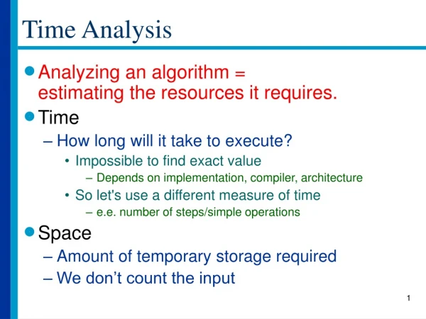
Time Analysis • Analyzing an algorithm = estimating the resources it requires. • Time • How long will it take to execute? • Impossible to find exact value • Depends on implementation, compiler, architecture • So let's use a different measure of time • e.e. number of steps/simple operations • Space • Amount of temporary storage required • We don’t count the input
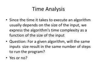
Time Analysis • Goals: • Compute the running time of an algorithm. • Compare the running times of algorithms that solve the same problem • Observations: • Since the time it takes to execute an algorithm usually depends on the size of the input, we express the algorithm'stime complexity as a function of the size of the input.
Time Analysis • Observations: • Since the time it takes to execute an algorithm usually depends on the size of the input, we express the algorithm'stime complexity as a function of the size of the input. • Two different data sets of the same size may result in different running times • e.g. a sorting algorithm may run faster if the input array is already sorted. • As the size of the input increases, one algorithm's running time may increase much faster than another's • The first algorithm will be preferred for small inputs but the second will be chosen when the input is expected to be large.
Time Analysis • Ultimately, we want to discover how fast the running time of an algorithm increases as the size of the input increases. • This is called the order of growth of the algorithm • Since the running time of an algorithm on an input of size n depends on the way the data is organized, we'll need to consider separate cases depending on whether the data is organized in a "favorable" way or not.
Time analysis • Best case analysis • Given the algorithm and input of size n that makes it run fastest (compared to all other possible inputs of size n), what is the running time? • Worst case analysis • Given the algorithm and input of size n that makes it run slowest (compared to all other possible inputs of size n), what is the running time? • A bad worst-case complexity doesn't necessarily mean that the algorithm should be rejected. • Average case analysis • Given the algorithm and a typical, average input of size n, what is the running time?
Time Analysis • Iterative algorithms • Concentrate on the time it takes to execute the loops • Recursive algorithms • Come up with a recursive function expressing the time and solve it.
Example • Sorting algorithm: insertion sort • The idea: • Divide the array in two imaginary parts: sorted, unsorted • The sorted part is initially empty • Pick the first element from the unsorted part and insert it in its correct slot in the sorted part. • Do the insertion by traversing the sorted part to find where the element should be placed. Shift the other elements over to make room for it. • Repeat the process. • This algorithm is very efficient for sorting small lists
Example continued As we "move" items to the sorted part of the array, this imaginary wall between the parts moves towards the end of the array. When it reaches the edge, we are done!
Example continued Input: array A of size n Output: A, sorted in ascending order function InsertionSort(A[1..n]) begin for i:=2 to n item := A[i] j := i - 1 while (j > 0 and A[j] > item) A[j+1] := A[j] j := j - 1 end while A[j+1] := item end for end
Example continued Input: array A of size n Output: A, sorted in ascending order function InsertionSort(A[1..n]) begin for i:=2 to n item := A[i] j := i - 1 while (j > 0 and A[j] > item) A[j+1] := A[j] j := j - 1 end while A[j+1] := item end for end times executed n n-1 n-1 tj (tj-1) (tj-1) n-1 depends on input
Example continued • Best case for insertion sort • The best case occurs when the array is already sorted. Then, the while loop is not executed and the running time of the algorithm is a linear function of n. • Worst case for insertion sort • The worst case occurs when the array is sorted in reverse. Then, for each value of i, the while loop is executed i-1 times. The running time of the algorithm is a quadratic function of n. • Average case for insertion sort • On average, the while loop is executed i/2 times for each value of i. The running time is again a quadratic function of n (albeit with a smaller coefficient than in the worst case)
Algorithm Analysis • Observations • Some terms grow faster than others as the size of the input increases ==> these determine the rate of growth • Example 1: • In n2+4n , n2 grows much faster than n. We say that this is a quadratic function and concentrate on the term n2. • Example 2: • Both n2+4n and n2 are quadratic functions. They grow at approximately the same rate. Since they have the same rate of growth, we consider them "equivalent".
Algorithm Analysis • We are interested in finding upper (and lower) bounds for the order of growth of an algorithm.
Algorithm Analysis: Big Oh • A function f(n) is O(g(n)) if there exist constants c, n0>0such thatf(n) c·g(n)for all n n0 • What does this mean in English? • c·g(n) is an upper bound of f(n) for large n • Examples: • f1(n) = 3n2+2n+1 is O(n2) • f2(n) = 2n is O(n) • f3(n) = 3n+1 is also O(n) • f2(n) and f3(n) have the same order of growth. • f4(n) = 1000n3 is O(n10)
Algorithm Analysis: Big Oh • To show that f(n) is O(g(n)), • all you need to do is find appropriate values for the constants c, n0 • To show that f(n) is NOT O(g(n)), • start out by assuming that you have found constants c, n0 for which f(n) c·g(n) and • then try to reach a contradiction: show that f(n) cannot possibly be less than c·g(n) if n can be any integer greater than n0
Algorithm Analysis: Omega • A function f(n) is (g(n)) if there exist constants c,n0>0such that f(n) c·g(n)for allnn0 • What does this mean in English? • c·g(n) is a lower bound of f(n) for large n • Example: • f(n) = n2 is (n)
Algorithm Analysis: Theta • A function f(n) is (g(n)) if it is both O(g(n)) and (g(n)) , in other words: • There exist constants c1,c2,n>0 s.t. 0 c1 g(n) f(n) c2g(n)for allnn0 • What does this mean in English? • f(n) and g(n) have the same order of growth • indicates a tight bound. • Example: • f(n) = 2n+1 is (n)
Algorithm analysis, Examples Input: Collection of size n Output: The smallest difference between any two different numbers in the collection Algorithm: List all pairs of different numbers in the collection estimate=difference between values in first pair. for each remaining pair compute the difference between the two values if it is less than estimate set estimate to that difference return estimate
Algorithm analysis, Examples Input: Collection of size n Output: The smallest difference between any two different numbers in the collection Algorithm: estimate = infinity for each value v in the collection for each value uv if |u-v| < estimate estimate = |u-v| return estimate