TIME SERIES ANALYSIS

1. TIME SERIES ANALYSIS 13-01-2011

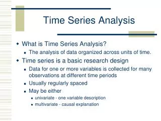
2. TIME SERIES ANALYSIS • Any series of observations ordered along a single dimension, such as time, may be thought of as a time series. The emphasis in time series analysis is on studying the dependence among observations at different points in time. What distinguishes time series analysis from general multivariate analysis is precisely the temporal order imposed on the observations

3. TIME SERIES ANALYSIS • Many economic variables, such as GNP and its components, price indices, sales, and stock returns are observed over time. In addition to being interested in the contemporaneous relationships among such variables, we are often concerned with relationships between their current and past values, i.e., relationships over time.

4. Some examples of time series

5. Geophysicaltime-series

6. 15 0 -15 15 0 -15 15 0 -15 4 2 0 -2 -4 -6 Observed Background Noise Seismic Signal Time-varying Variance (in log10) 0 400 800 1200 1600 2000 2400 2800

7. Chemical concentrations off the coast of south Texas

8. TIME SERIES ANALYSIS • STOCHASTIC PROCESSES • A random or stochastic process is a collection of random variables ordered in time. If we let Y denote a random variable, and if it is continuous, we denote it as y(t), but if it is discrete we denoted it as Yt. An example of the former is an electrocardiogram, and an example of the latter is GDP, PDI, etc.

9. TIME SERIES ANALYSIS • Since most economic data are collected at discrete points in time, for our purpose we will use the notation Yt rather than Y(t).

10. TIME SERIES ANALYSIS • Stationary Stochastic Processes • A type of stochastic process that has received a great deal of attention and scrutiny by time series analysts is the so-called stationary stochastic process. Broadly speaking, a stochastic process is said to be stationary if its mean and variance are constant over time and the value of the covariance between the two time periods depends only on the distance or gap or lag between

11. TIME SERIES ANALYSIS the two time periods and not the actual time at which the covariance is computed. In the time series literature, such a stochastic process is known as a weakly stationary, or covariance stationary, or second-order stationary, or wide sense, stochastic process.

12. TIME SERIES ANALYSIS • To explain weak stationarity, let Yt be a stochastic time series with these properties: • Mean: E(Yt) = μ • Variance: var (Yt) = E(Yt − μ)2 = σ2 • Covariance: γk = E[(Yt − μ)(Yt+k − μ)]

13. TIME SERIES ANALYSIS • In short, if a time series is stationary, its mean, variance, and autocovariance (at various lags) remain the same no matter at what point we measure them; that is, they are time invariant. Such a time series will tend to return to its mean (called mean reversion) and fluctuations around this mean (measured by its variance) will have a broadly constant amplitude. • If a time series is not stationary in the sense just defined, it is called a nonstationary time series (keep in mind we are talking only about weak stationarity). In other words, a nonstationary time series will have a timevarying mean or a time-varying variance or both.

14. TIME SERIES ANALYSIS • Nonstationary Stochastic Processes • Although our interest is in stationary time series, one often encounters nonstationary time series, the classic example being the random walk model (RWM). It is often said that asset prices, such as stock prices or exchange rates, follow a random walk; that is, they are nonstationary.

15. TIME SERIES ANALYSIS • We distinguish two types of random walks: (1) random walk without drift (i.e., no constant or intercept term) and (2) random walk with drift (i.e., a constant term is present). • Random Walk without Drift. Suppose ut is a white noise error termwith mean 0 and variance σ2. Then the series Yt is said to be a random walk if Yt = Yt−1 + ut (1)

16. TIME SERIES ANALYSIS • Random Walk with Drift. Let us modify (1) as follows: Yt = α + Yt−1 + ut • where α is known as the drift parameter. The name drift comes from the fact that if we write the preceding equation as Yt − Yt−1 = Yt = α + ut

17. TIME SERIES ANALYSIS • it shows that Ytdrifts upward or downward, depending on α being positive or negative. Note that model is also an AR(1) model.

18. UNIT ROOT STOCHASTIC PROCESS • Let us write the RWM as Yt = ρYt−1 + ut -1 ≤ρ ≤ 1 • This model resembles the Markov first-order autoregressive model. If ρ = 1, (1) becomes a RWM (without drift). If ρ is in fact 1, we face what is known as the unit root problem, that is, a situation of nonstationarity;

19. TIME SERIES ANALYSIS • we already know that in this case the variance of Yt is not stationary. The name unit root is due to the fact that ρ = 1. Thus the terms nonstationarity, random walk, and unit root can be treated as synonymous.

20. TREND STATIONARY (TS) AND DIFFERENCE STATIONARY (DS) STOCHASTIC PROCESSES • if the trend in a time series is completely predictable and not variable, we call it a deterministic trend, whereas if it is not predictable, we call it a stochastic trend.

21. Yt = β1 + β2t + β3Yt−1 + ut (1) • where ut is a white noise error term and where t is time measured chronologically.

22. Pure random walk: If in (1) β1 = 0, β2 = 0, β3 = 1, we get Yt = Yt−1 + ut(2) which is nothing but a RWM without drift and is therefore nonstationary. But note that, if we write (2) as Yt = (Yt − Yt−1) = ut it becomes stationary, as noted before. Hence, a RWM without drift is a difference stationary process (DSP).

23. Random walk with drift: If in (1) β1≠ 0, β2 = 0, β3 = 1, we get Yt = β1 + Yt−1 + ut(3) • which is a random walk with drift and is therefore nonstationary. If we write it as (Yt − Yt−1) = Yt = β1 + ut(3a) this means Yt will exhibit a positive (β1 > 0) or negative (β1 < 0) trend . Such a trend is called a stochastic trend.

24. Equation (3a) is a DSP process because the nonstationarity in Yt can be eliminated by taking first differences of the time series.

25. Deterministic trend: If in (1), β1≠0, β2≠0, β3 = 0, we obtain Yt = β1 + β2t + ut(4) • which is called a trend stationary process (TSP). Although the mean of Ytis β1 + β2t, which is not constant, its variance ( = σ2) is. Once the values of β1 and β2 are known, the mean can be forecast perfectly.

26. Therefore, if we subtract the mean of Yt from Yt, the resulting series will be stationary, hence the name trend stationary.

27. Random walk with drift and deterministic trend: If in (1), β1≠0, β2≠ 0, β3 = 1, we obtain: Yt = β1 + β2t + Yt−1 + ut(5) • we have a random walk with drift and a deterministic trend, which can be seen if we write this equation as Yt = β1 + β2t + ut(5a) which means that Yt is nonstationary.

28. Deterministic trend with stationary AR(1) component: If in (1) β1≠0, β2≠ 0, β3 < 1, then we get Yt = β1 + β2t + β3Yt−1 + ut(6) which is stationary around the deterministic trend.

29. INTEGRATED STOCHASTIC PROCESSES • The specific case of a more general class of stochastic processes known as integrated processes. Recall that the RWM without drift is nonstationary, but its first difference, is stationary. Therefore, we call the RWM without drift integrated of order 1, denoted as I(1).

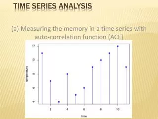
30. TESTS OF STATIONARITY • Graphical Analysis • Autocorrelation Function (ACF) and Correlogram • Statistical tests

31. Autocorrelation Function (ACF) and Correlogram • The ACF at lag k denoted by • Where is covariance at lag k and is variance.

32. A plot of against k is known as the sample Correlogram.

33. Statistical Significance of Autocorrelation Coefficients • As ρˆk ∼ N(0, 1/n) • The 95% C.I for ρk

34. Using Q statistic (Box and pierce) • where n = sample size and m = lag length.

35. Ljung-Box statistic

36. The Choice of Lag Length • A rule of thumb is to compute ACF up to one-third to one-quarter the length of the time series. • Using statistical criterion of selection of lags • Akiake information criterion (AIC) • Bayesian information criterion (BIC)

38. THE UNIT ROOT TEST (test for stationarity) Yt = ρYt−1 + ut (1) where ut is a white noise error term. • We know that if ρ = 1, that is, in the case of the unit root, (1) becomes a random walk model without drift, which we know is a nonstationary stochastic process.

39. Simply regress Yt on its (one period) lagged value Yt−1 and find out if the estimated ρ is statistically equal to 1? If it is, then Yt is nonstationary. Now subtract Yt-1 from (1), Yt − Yt−1 = ρYt−1 − Yt−1 + ut = (ρ − 1)Yt−1 + ut

40. which can be written as: Yt =δYt−1 + ut (2) • Where δ= (ρ − 1). • First estimate (2) and then test the hypothesis that δ=0 , that is we have a unit root. This means that time series under consideration is nonstationary.

41. If δ=0 then • Yt = (Yt − Yt−1) = ut • As ut is white noise term, it is stationary, which means that the 1st difference of random walk time series are stationary.

42. Dickey–Fuller (DF) test Yt is a random walk: Yt = δYt−1 + ut Yt is a random walk with drift: Yt = β1 + δYt−1 + ut Yt is a random walk with drift around a stochastic trend: Yt = β1 + β2t + δYt−1 + ut

43. The Augmented Dickey–Fuller (ADF) Test • Yt = β1 + β2t + δYt−1 +∑αiYt−i+ εt

44. Exponential Smoothing: This is a very popular scheme to produce a smoothed Time Series. Whereas in Moving Averages the past observations are weighted equally, Exponential Smoothing assigns exponentially decreasing weights as the observation get older. In other words, recent observations are given relatively more weight in forecasting than the older observations. Double Exponential Smoothing is better at handling trends. Triple Exponential Smoothing is better at handling parabola trends.

45. An exponenentially weighted moving average with a smoothing constant a, corresponds roughly to a simple moving average of length (i.e., period) n, where a and n are related by: • a = 2/(n+1)    OR    n = (2 - a)/a. • Thus, for example, an exponenentially weighted moving average with a smoothing constant equal to 0.1 would correspond roughly to a 19 day moving average. And a 40-day simple moving average would correspond roughly to an exponentially weighted moving average with a smoothing constant equal to 0.04878.