Example II: Linear truss structure

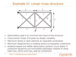
1. Example II: Linear truss structure • Optimization goal is to minimize the mass of the structure • Cross section areas of trusses as design variables • Maximum stress in each element as inequality constraints • Maximum displacement in loading points as inequality constraints • Gradient-based and ARSM optimization perform much better if constraint equations are formulated separately instead of using total max_stress and max_disp as constraints Part 4: Multidisciplinary Optimization

2. Example II: Sensitivity analysis • MOP indicates only a1, a3, a8 as important variables for maximum stress and displacements,but all inputs are important for objective function Part 4: Multidisciplinary Optimization

3. Example II: Sensitivity analysis a1 a2 a3 a4 a5 a6 a7 a8 a9 a10 max_stress max_disp stress10 stress9 stress8 stress8 stress6 stress5 stress4 stress3 stress2 stress1 disp4 disp2 mass MOP filter • For single stress values used in constraint equations, each input variable occurs at least twice as important parameter • Reduction of number of inputs seems not possible Part 4: Multidisciplinary Optimization

4. Example II: Gradient-based optimization • Best design with valid constraints: mass = 1595 (19% of initial mass) • Areas of elements 2,5,6 and 10 are set to minimum • Stresses in remaining elements reach maximum value • 153 solver calls (+100 from DOE) Part 4: Multidisciplinary Optimization

5. Example II: Adaptive response surface • Best design with valid constraints: mass = 1613 (19% of initial mass) • Areas of elements 2,6 and are set to minimum, 5 and 10 are close to minimum • 360 solver calls Part 4: Multidisciplinary Optimization

6. Example II: EA (global search) • Best design with valid constraints: mass = 2087 (25% of initial mass) • 392 solver calls Part 4: Multidisciplinary Optimization

7. Example II: EA (local search) • Best design with valid constraints: mass = 2049 (24% of initial mass) • 216 solver calls (+392 from global search) Part 4: Multidisciplinary Optimization

8. Example II: Overview optimization results • NLPQL with small differentiation interval with best DOE as start design is most efficient • Local ARSM gives similar parameter set • EA/GA/PSO with default settings come close to global optimum • GA with adaptive mutation has minimum constraint violation Part 4: Multidisciplinary Optimization

9. When to use which optimization algorithms • Gradient-based algorithms • Most efficient method if gradients are accurate enough • Consider its restrictions like local optima, only continuous variablesand noise • Response surface method • Attractive method for a small set of continuous variables (<15) • Adaptive RSM with default settings is the method of choice • Biologic Algorithms • GA/EA/PSO copy mechanisms of nature to improve individuals • Method of choice if gradient or ARSM fails • Very robust against numerical noise, non-linearities, number of variables,… Start Part 4: Multidisciplinary Optimization

10. Sensitivity Analysis and Optimization 1) Start with a sensitivity study using the LHS Sampling • 2) Identify the important parameters and responses • understand the problem • reduce the problem Scan the whole Design Space Understand the Problem using CoP/MoP optiSLang Search for Optima 3) Run an ARSM, gradient based or biological based optimization algorithm 4) Goal: user-friendly procedure provides as much automatism as possible Part 4: Multidisciplinary Optimization

11. Optimization of a Large Ship Vessel • Optimization of the total weight of two load cases with constrains (stresses) • 30.000 discrete Variables • Self regulating evolutionary strategy • Population of 4, uniform crossover for reproduction • Active search for dominant genes with different mutation rates Solver: ANSYS Design Evaluations: 3000 Design Improvement: > 10 % EVOLUTIONARY ALGORITHM Part 4: Multidisciplinary Optimization

12. Optimization of passive safety Adaptive Response Surface Methodology • Optimization of passive safety performance US_NCAP & EURO_NCAP • using Adaptive Response Surface Method • 3 and 11 continuous variables • weighted objective function • Solver: MADYMO Design Evaluations: 75 Design Improvement: 10 % Part 4: Multidisciplinary Optimization

13. Solver: ANSYS (using automatic spot weld Meshing procedure) Design evaluations: 200 Design improvement: 47% 134 binary variables, torsion loading, stress constrains Weak elitism to reach fast design improvement Fatigue related stress evaluation in all spot welds Genetic Optimization of Spot Welds Part 4: Multidisciplinary Optimization

14. Optimization of an Oil Pan The intention is to optimize beads to increase the first eigenfrequency of an oil pan by more than 40%. Topology optimization indicate possibility > 40% improvement, but test failed. Sensitivity study and parametric optimization using parametric CAD design + ANSYS workbench+optiSLang could solve the task. Initial design beads design after topology optimization beads design after parameter optimization Design Parameter 50 Design Evaluations: 500 CAE: ANSYS workbench CAD: Pro/ENGINEER [Veiz. A; Will, J.: Parametric optimization of an oil pan; Proceedings Weimarer Optimierung- und Stochastiktage 5.0, 2008] Part 4: Multidisciplinary Optimization

15. Several optimization criteria are formulated in terms of the input variables x Strategy A: Only the most important objective function is used as optimization goal Other objectives as constraints Strategy B: Weighting of single objectives Multi Criteria Optimization Strategies Part 4: Multidisciplinary Optimization

16. Example: damped oscillator • Objective 1: minimize maximum amplitude after 5s • Objective 2: minimize eigen-frequency • DOE scan with 100 LHS samples gives good problem overview • Weighted objectives require about 1000 solver calls Part 4: Multidisciplinary Optimization

17. Multi Criteria Optimization Strategies Strategy C: Pareto Optimization Part 4: Multidisciplinary Optimization

18. Multi Criteria Optimization Strategies Design space Objective space • Only for conflicting objectives a Pareto frontier exists • For positively correlated objective functions only one optimum exists Part 4: Multidisciplinary Optimization

19. Multi Criteria Optimization Strategies Conflicting objectives Correlated objectives Part 4: Multidisciplinary Optimization

20. Multi Criteria Optimization Strategies Pareto dominance • Solution a dominates solution c since a is better in both objectives • Solution a is indifferent to b since each solution is better than the respective other in one objective (a dominates c) (a is indifferent to b) Part 4: Multidisciplinary Optimization

21. Multi Criteria Optimization Strategies Pareto optimality • A solution is called Pareto-optimal if there is no decision vector that would improve one objective without causing a degradation in at least one other objective • A solution a is called Pareto-optimal in relation to a set of solutions A, if it is not dominated by any other solution c Requirements for ideal multi-objective optimization • Find a set of solutions close to the Pareto-optimal solutions (convergence) • Find solutions which are diverse enough to represent the whole Pareto front (diversity) Part 4: Multidisciplinary Optimization

22. Multi Criteria Optimization Strategies Pareto Optimization using Evolutionary Algorithms • Only in case of conflicting objectives, a Pareto frontier exists and Pareto optimization is recommended (optiSLang post processing supports 2 or 3 conflicting objectives) • Effort to resolute Pareto frontier is higher than to optimize one weighted optimization function Part 4: Multidisciplinary Optimization

23. Example: damped oscillator • Pareto optimization with EA gives good Pareto frontier with 123 solver calls Part 4: Multidisciplinary Optimization

24. Example II: linear truss structure Anthill plot from ARSM Pareto front 1. • For more complex problems the performance of the Pareto optimization can be improved if a good start population is available • This can be found in selected designs of a previous DOE or single objective optimization Part 4: Multidisciplinary Optimization

25. Optimization Algorithms Local adaptive RSM Biologic Algorithms Genetic algorithms, Evolutionary strategies & Particle Swarm Optimization Gradient-based algorithms Start Response surface method (RSM) Global adaptive RSM Pareto Optimization Part 4: Multidisciplinary Optimization