Linear Mixed Models: An Introduction
Linear Mixed Models: An Introduction. Patrick J. Rosopa, Ph.D. University of Central Florida. Outline. The Need for Linear Mixed Models General Linear Models versus Linear Mixed Models A Quick Note Regarding Software Types of Effects Some Common Models Estimation of Parameters


Linear Mixed Models: An Introduction
E N D
Presentation Transcript
Linear Mixed Models:An Introduction Patrick J. Rosopa, Ph.D. University of Central Florida
Outline • The Need for Linear Mixed Models • General Linear Models versus Linear Mixed Models • A Quick Note Regarding Software • Types of Effects • Some Common Models • Estimation of Parameters • Goodness-of-Fit Indices • Statistical Inferences • Covariance Structures • Linear Mixed Models in SPSS • Some Examples Using SPSS
Grouped Data is Common • In the social and behavioral sciences, including industrial and organizational psychology, grouped or clustered data is quite common (Hox, 2002; Raudenbush & Bryk, 2002). • Team members nested within teams. • Students nested within schools. • Employees nested within departments & departments within organizations. • Interviewees nested within interviewer. • Randomized block designs. • In longitudinal and growth curve research, several repeated measurements are nested within individuals. • In meta-analysis, participants are nested within different studies.
Person 1 Score time1 Score time2 Score time3
To Aggregate or Not to Aggregate? • In some situations, all variables are aggregated to the “higher” level (e.g., team, school). • In some situations, all variables are disaggregated to the “lower” level (e.g., team member, student). • In both, ordinary least squares (OLS) “fixed effects” general linear models are frequently used. (regression or ANOVA of some kind)
To Aggregate or Not to Aggregate? • In some situations, all variables are aggregated to the “higher” level (e.g., team, school).
Compute Mean Compute Mean
To Aggregate or Not to Aggregate? • In some situations, all variables are aggregated to the “higher” level (e.g., team, school). • Result: Within-group information is lost, smaller sample size, and loss of statistical power.
To Aggregate or Not to Aggregate? • In some situations, all variables are aggregated to the “higher” level (e.g., team, school). • Result: Within-group information is lost, smaller sample size, and loss of statistical power. • In some situations, all variables are disaggregated to the “lower” level (e.g., team member, student).
To Aggregate or Not to Aggregate? • In some situations, all variables are aggregated to the “higher” level (e.g., team, school). • Result: Within-group information is lost, smaller sample size, and loss of statistical power. • In some situations, all variables are disaggregated to the “lower” level (e.g., team member, student). • Result: Observations are treated as if they were independent when they really aren’t, resulting in overly optimistic (i.e., smaller) standard errors and increased Type I error rate. (unjustified increase in power)
Linear Mixed Models as a Solution • Linear mixed models used to account for: • the lack of independence, i.e., correlation, among observations • the unequal errors, i.e., heteroscedasticity, across observations (non-constant variance across groups) • both lack of independence and heteroscedasticity across observations • Additional advantages: • It can handle missing values and will not drop cases from the analysis (unlike standard repeated measures ANOVA). • Time can be treated flexibly (Singer & Willett, 2003). (e.g., One person measured on the dependent variable at Time 1, Time 4, & Time 6. Another person measured at Time 1, Time 3, Time 5, & Time 6.). • When used in Generalizability Theory, the common estimation methods (i.e., ML & REML, to be discussed later) will not result in negative variance components.
Linear Mixed Models as a Solution • “The Linear Mixed Models procedure expands the general linear model so that the error terms and random effects are permitted to exhibit correlated (non independent) and non-constant variability (heteroscedasticity). The linear mixed model, therefore, provides the flexibility to model not only the mean of a response variable, but its covariance structure as well.” (SPSS, 2006)
General Linear Models vs.Linear Mixed Models • How does a traditional general linear model (GLM) differ from a linear mixed model (LMM)? • Some traditional GLMs: • Analyses involving the mean of a single group (1 sample t test) • Analyses involving the means of 2 independent groups (1 categorical IV) • Analyses involving the means of > 2 independent groups (1 categorical IV) • Factorial designs (2 or more completely crossed categorical IVs) • Multiple regression (continuous IVs) • ANCOVA (continuous and categorical IVs), etc. y = (Fixed Effects) + random error
General Linear Models vs.Linear Mixed Models GLM: y = (Fixed Effects) + random error LMM: y = (Fixed Effects) + (Random Effects) + random error • When there are no random effects, we have the usual fixed effects general linear model (Pinheiro & Bates, 2000; Searle, Casella, & McCulloch, 1992). This model is covered in detail by numerous researchers (Cohen, Cohen, West, & Aiken, 2003; Fox, 1997; Pedhazur, 1982).
Some Terminology • Linear mixed models, hierarchical linear models (psych), multilevel models (edu, and psych), and random coefficient models are used interchangeably. • Note that these are computed using a model that incorporates fixed and/or random effects; thus, major software packages use “mixed” or “mixed effects.” • SPSS procedure: MIXED. • SAS procedure: PROC MIXED. • S-PLUS function: lme. (linear mixed effects) • R function: lme.
General-Purpose Statistical Software • Able to fit linear mixed models.
MLwiN Specialized Statistical Software • Developed specifically for linear mixed models.
Fixed vs. Random Effects • Fixed effects: used to model the mean or predicted value of Y. The levels or values of the predictor are not sampled from a larger population. • Sex • Ethnicity • Fixed effects take the form of the usual regression coefficients, e.g., standardized or unstandardized. (slopes and intercepts) • In the literature on hierarchical linear modeling, random coefficient modeling, and multilevel modeling, the fixed effects are typically denoted by gammas (γ) instead of betas (β). • As in general linear models, you will be able to obtain the correlation and/or covariance matrix among the fixed effects coefficients in SPSS.
Fixed vs. Random Effects • Random effects: used to account for the variance-covariance of DV after the fixed effects have been accounted for (of Y). The levels or values observed have been sampled from a larger population of possible levels or values. • Teams • Schools • Persons (in longitudinal studies) • Clinics (e.g., selecting a representative sample of clinics to test for the effectiveness of a new procedure) • Blocks (in a randomized block design)
Fixed vs. Random Effects • In the literature on hierarchical linear modeling, random coefficient modeling, and multilevel modeling, the random effects are denoted by u. • Instead of e for residuals or ε for errors, r is used. • Creating an interaction term that involves both a fixed effect AND a random effect results in a random effect term. • e.g., the interaction between a fixed effect term (sex) and random effect term (Team ID) results in a random effect term (sex × Team ID). • In statistical software, you will be able to obtain the correlation and/or covariance matrix among the random effects. • e.g., If you have 2 random effects, there will be a 2 × 2 covariance matrix for the random effects. This contains the estimated variance components.
Null Model • Also called the fully unconditional model (Raudenbush & Bryk, 2002). • In the experimental design literature, it is known as a one-way random effects ANOVA (Kirk, 1995). • Most basic model you can fit for a linear mixed model • No predictors
Null Model • Also called the fully unconditional model (Raudenbush & Bryk, 2002). • In the experimental design literature, it is known as a one-way random effects ANOVA (Kirk, 1995). Level 1: Level 2: LMM:
Null Model • Also called the fully unconditional model (Raudenbush & Bryk, 2002). • In the experimental design literature, it is known as a one-way random effects ANOVA (Kirk, 1995). Mean in jth School/Team/Cluster Level 1: Level 2: LMM:
Null Model • Also called the fully unconditional model (Raudenbush & Bryk, 2002). • In the experimental design literature, it is known as a one-way random effects ANOVA (Kirk, 1995). Level 1: Grand Mean, that is, . . . Level 2: LMM:
Null Model • Also called the fully unconditional model (Raudenbush & Bryk, 2002). • In the experimental design literature, it is known as a one-way random effects ANOVA (Kirk, 1995). Level 1: Level 2: LMM: Fixed Effect (Intercept)
Null Model • Also called the fully unconditional model (Raudenbush & Bryk, 2002). • In the experimental design literature, it is known as a one-way random effects ANOVA (Kirk, 1995). Level 1: Level 2: LMM: Random Effect for jth School/Team/Cluster
Null Model • Also called the fully unconditional model (Raudenbush & Bryk, 2002). • In the experimental design literature, it is known as a one-way random effects ANOVA (Kirk, 1995). Level 1: Level 2: LMM: Residual
Null Model • From this model, we can estimate the intraclass correlation (ICC(1,1)), Shrout & Fleiss, 1979) or cluster effect (Raudenbush & Bryk, 2002; Snijders & Bosker, 2003). • A large value suggests that differences between schools/teams/clusters are larger than differences within them. Inappropriate to treat observations within the same school/team/cluster as independent. LMM:
Null Model • We can also use the variance component from the null model to determine whether we can explain additional variability between schools/teams/clusters by including additional variables. Proportion of Explained Variance
Adding a Fixed Effect from Level 2 • Adds a predictor • First example had one fixed effect (i.e., the intercept) and one random effect due to the school/team/cluster. • We could add a fixed effect from Level 2 (e.g., a predictor on which we have the mean within the group, a team characteristic).
Adding a Fixed Effect from Level 2 • First example had one fixed effect (i.e., the intercept) and one random effect due to the school/team/cluster. • We could add a fixed effect from Level 2 (e.g., a predictor on which we have the mean within the group, a team characteristic). Level 1: Level 2: LMM: Fixed Effect (Intercept) Fixed Effect (Slope)
Adding a Fixed Effect from Level 2 • First example had one fixed effect (i.e., the intercept) and one random effect due to the school/team/cluster. • We could add a fixed effect from Level 2 (e.g., a predictor on which we have the mean within the group, a team characteristic). Level 1: Level 2: LMM: Random Effect for jth School/Team/Cluster
Adding a Fixed Effect from Level 2 • First example had one fixed effect (i.e., the intercept) and one random effect due to the school/team/cluster. • We could add a fixed effect from Level 2 (e.g., a predictor on which we have the mean within the group, a team characteristic). Level 1: Level 2: LMM: Residual
Adding a Fixed Effect from Level 1 • First example had one fixed effect (i.e., the intercept) and one random effect due to the school/team/cluster. • We could add a fixed effect from Level 1 (e.g., a predictor on which we have values that vary within a group, but are not sampled from a larger population).
Adding a Fixed Effect from Level 1 Level 1: Level 2: LMM:
Adding a Fixed Effect from Level 1 Level 1: Level 2: LMM: Fixed Effect (Intercept) Fixed Effect (Slope)
Adding a Fixed Effect from Level 1 Level 1: Level 2: LMM: Random Effect for jth School/Team/Cluster
Adding a Fixed Effect from Level 1 Level 1: Level 2: LMM: Residual
Adding a Fixed Effect Covariate from Level 1 • First example had one fixed effect (i.e., the intercept) and one random effect due to the school/team/cluster. • Add a fixed effect covariate from Level 1 (e.g., cognitive ability scores which have values that vary within a group, but are not sampled from a larger population). • This is a one-way ANCOVA with a random effect for the school/team/cluster.
Adding a Fixed Effect Covariate from Level 1 Level 1: Level 2: LMM: