PART 4 Non-linear models
PART 4 Non-linear models. Logistic regression Other non-linear models Generalized Estimating Equations (GEE) Examples Crossover study British Social Attitudes Survey. Models for Clustered Data. Inferential goals Marginal mean/Population Averaged

PART 4 Non-linear models
E N D
Presentation Transcript
PART 4 Non-linear models • Logistic regression • Other non-linear models • Generalized Estimating Equations (GEE) • Examples • Crossover study • British Social Attitudes Survey BIO656--Multilevel Models
Models for Clustered Data Inferential goals • Marginal mean/Population Averaged • Average response across “the population” • Mean, conditional on • Other responses in the cluster • Unobserved random effects BIO656--Multilevel Models
Interpreting Linear Model Coefficients Same interpretation for conditional (cluster-specific) and population-averaged inferences • Unit change in dependent variable for a unit change in regressor • Multi-level models specify correlations and latent effects: • The random intercept model produces an equal-correlation model (correlation • The latent intercepts can be estimated and used for prediction BIO656--Multilevel Models
Marginal Models Inferential Target • Marginal mean or population-averaged response for different values of predictor variables Examples • Difference in mean alcohol consumption for two age groups • Rate of alcohol abuse for states with addiction treatment programs compared to those without Public health assessments BIO656--Multilevel Models
Conditional Models Conditional on other observations in cluster • Probability that a person abuses alcohol given family membership or given the number of family members that do • Probability that a person will abuse next year, if abuses this year • A person’s average alcohol consumption given the average in the neighborhood BIO656--Multilevel Models
Conditional Models Conditional on random effects • Average consumption, conditional on a latent tendency • Probability that a person abuses alcohol, conditional on a latent tendency Can be thought of as conditional on unmeasured covariates BIO656--Multilevel Models
The basic, conditional logistic model • Conditional on a random effect, you have the logistic regression: logit(P) = log{P/(1-P)} = u + + X u ~ (0, 2) Implications • Generally, the population averaged (marginal) model will not have the logistic shape • In any case, the slope on a covariate will have a different impact in the conditional and marginal models BIO656--Multilevel Models
Condition on u BIO656--Multilevel Models
Conditional Logistic and Marginal ShapesU N(0, 4) u=0 b = BIO656--Multilevel Models
Conditional Logistic and Marginal ShapesU is a two-point mixture at 2 u=0 b = BIO656--Multilevel Models
Adjust the conditional slope to closely match the marginal curve • Assume that there is a population relation that is logistic with term X • How far off is the marginal curve produced from the conditional logistic curve with term X? • Let * be the slope needed in the conditional logistic so that the marginal curve produced from it comes close to the population relation • “Comes close” means to track the middle part of the population curve BIO656--Multilevel Models
Non-linear model coefficients • Usually, population-averaged (marginal) and conditional models have different shapes • Condition logistic is not population logistic • But, conditional probit is population probit • In any case, population-averaged and cluster-specific coefficients have different magnitudes and interpretations because they address different questions • For example, when u is a two-point, 50/50 mixture at 2, = 4 and * = 8. Need to consider impact on probabilities not just on odds ratios BIO656--Multilevel Models
SHAPE & SLOPE CHANGES • For linear models, regression coefficients in random effects models and marginal models are identical: average of linear model = linear model of average • For non-linear models, coefficients have different meanings and values: average of non-linear model non-linear model of average coefficient value and meaning in average model coefficient value and meaning in conditional model BIO656--Multilevel Models
Conditional Logistic and Marginal Shapes Log(odds | u) = u -2.0 + 0.4X Population prevalences X = 1 X = 0 Cluster-specific probabilities BIO656--Multilevel Models
Logistic Regression Example Cross-over trial 2 observations per person (before/after) Response 1=not alcohol dependent; 0 = AlcDep (so a high probability is good!) Predictors period (Pd = 0 or 1) treatment group (Trt = 0 or 1) Parameter of interest • Treatment vs placebo after/before log(OddsRatio) • A positive slope favors the treatment BIO656--Multilevel Models
Baseline/Follow-up Model i = period, j = person; logit(P) = log(P/[1-P]) Population level (no individual effects) logit(Pij) = + 1PDij + 2TRij + 3PDijTR2ij = + 1PDi + 2TRj + 3PDiTRj logit(P2j) - logit(P1j) = 1+ 3TRj (3 is the treatment effect) Person-level (individual intercept) logit(Pij) = uj + * + *1PDi + *2TRj + *3PDiTRj uj ~ (0, 2) BIO656--Multilevel Models
Results for population-level regressions(logistic without multi-level component) Similar estimates; wrong standard error for Std. Logistic BIO656--Multilevel Models
The effect of accounting for correlation • Treatment effect estimates are the same for marginal logistic and correlation accounted logistic • But, SEs are 0.38 and 0.23 respectively • Why is the second smaller than the first? Answer • The treatment effect is estimated by contrasting (differencing) period 2 and period 1 • The positive, within-person correlation produces a smaller variance of this difference than does assuming independence BIO656--Multilevel Models
Population-level vs Random Intercept logistic regressionslog(OR)(se) BIO656--Multilevel Models
Marginal Logistic versusRandom Intercept Logistic Unconditional Logistic (Population-level inference): The population AlcnonDep(after/before), treatment/placebo prevalence odds ratiois exp(0.57) = 1.77 Conditional, RE Logistic (Individual-level inference): An individual’sAlcnonDep (after/before), treatment/placebo prevalence odds ratio is exp(1.80) = 6.05 Ratio: (Conditional)/(Marginal) 6.05/1.77 = 3.42 (= e1.23; 1.23 = 1.80-0.57) Different questions; different (but compatible) answers BIO656--Multilevel Models
Consequence of Conditional/Marginal Slope Differences • A population-level analysis that does not build on a multi-level model (that does not include the random effect) can understate the individual-level (cluster level) risk or benefit • Understate environmental risk • Understate benefits of lowering blood pressure • ......... BIO656--Multilevel Models
Relation between marginal and conditional ORs logit(pr(Y = 1 | X, u) = u + log(3)X u = log(3) with probability 1/2 3.00= (.5/.5)(.25/.75) = (.9/.1) (.75/.25) BIO656--Multilevel Models
u as a missing covariate • Without knowing u, a marginal logistic regression predicts 0.50 and 0.70 for X=0 and X=1 respectively • The log(OR) slope on X is 0.847 = log(2.333) • If we know u, a logistic regression with it as a covariate (conditional on it) predicts as in the table • The log(OR) slope on X is 1.099 = log(3.00) BIO656--Multilevel Models
Conditional Logistic and Marginal Shapes Log(odds | u) = u + X u > 0 u < 0 X BIO656--Multilevel Models
The RE induces association (Y1, Y2) are in the same cluster The RE model produces the following 22 table for X = 0 5/16 = [(3/4)(3/4) + (1/4)(1/4)]2 pr(Y2 =1 | Y1 = 0) = 3/8 = 3/(3+5) pr(Y2 =1 | Y1 = 1) = 5/8 = 5/(3+5) BIO656--Multilevel Models
The RE induces association (Y1, Y2) are in the same cluster The RE model produces the following 22 table for X = 1 13/100 = [(1/2)(1/2) + (1/10)(1/10)]2 pr(Y2 =1 | Y1 = 0) = 17/30 = 17/(17+13) pr(Y2 =1 | Y1 = 1) = 53/70 = 53/(17+53) BIO656--Multilevel Models
Updating the distribution of u For X = 1 (you can try it for X = 0) pr(u = +log(3) | Y = 0) = pr(u = +log(3), Y = 0)/pr(Y = 0) = (1/2)(1/10)(3/10) = 1/6 < 0.5 pr(u = +log(3) | Y = 1) = pr(u = +log(3), Y = 1)/pr(Y = 1) = (1/2)(9/10)(7/10) = 9/14 > 0.5 pr(u = +log(3)) = (1/6)(3/10) + (9/14)(7/10) = 0.5 Can use these to get [Y2 | Y1] BIO656--Multilevel Models
Marginal Multi-level, non-linear Models GEE: Marginal mean as a function of covariates • Working independence or other working model • Followed by Robust SE • “Cluster(id) in Stata • “Robust” Option in SAS Proc Mixed or GenMod • No “robustness” in BUGS Conditional mean, as a function of marginal mean and cluster-specific random effects • Heagerty (1999, Biometrics) • Heagerty and Zeger (2000, Statistical Science) BIO656--Multilevel Models
Generalized Linear Models (GLMs)g(mean) = 0 + 1 X1 + ... + p Xp(always a marginal model) BIO656--Multilevel Models
Baseline/Follow-up Model i = period, j = person; logit(P) = log(P/[1-P]) Population level (no individual effects) logit(Pij) = + 1PDij + 2TRij + 3PDijTR2ij = + 1PDi + 2TRj + 3PDiTRj logit(P2j) - logit(P1j) = 1+ 3TRj (3 is the treatment effect) Person-level (individual intercept) logit(Pij) = uj + * + *1PDi + *2TRj + *3PDiTRj uj ~ (0, 2) BIO656--Multilevel Models
Marginal Generalized Linear Modelsvia Generalized Estimating Equations (GEE) • Ordinary GLM (linear, logistic, Poisson,..) • Population-average parameters • Logit: Oij = logit(pij) = 0 + 1Xij • Then, model association among observations i and i’ in cluster j: corr(log(Oij/ Oi’j))= function(G) • Solve generalized estimating equation (GEE) • Diggle, Heagerty, Liang and Zeger, 2002) • Gives highly efficient and valid inferences on population-average parameters BIO656--Multilevel Models
Marginal Models for the Cross-Over Studylog(OR) Estimation method has an effect BIO656--Multilevel Models
Conditional (RE) Models for the Cross-Over Studylog(OR) BIO656--Multilevel Models
Accounting for Clusteringvia Sample Reuse Standard GEE: “Robust” option in SAS Jackknife • Compute hat • Delete aperson (in general, a “unit”) • Compute -i i = 1, ..., n • Compute i* = nhat - (n-1) -i • Compute the sampe (co)variance of the i* Bootstrap • Put each person’s data on a token • Sample “n” tokens with replacement and compute estimates from the sample • Do this “Nboot” times and compute sample (co)variance of the estimates • Can get more sophisticated CIs, via BCa BIO656--Multilevel Models
FRAMEWORK FOR SAMPLE REUSE Estimate Data “Black Box” Procedure BIO656--Multilevel Models
British Social Attitudes Survey: Conditional and Marginal MLMsNote:Subscript order reversed from our usual Response • Yijk = 1 if favor abortion; 0 if not • district i = 1,…264 • person j = 1,…,1056 • year k = 1, 2, 3, 4 Levels • Time within person • Persons within districts • Districts BIO656--Multilevel Models
Covariates at the three levels Level 1: time • Indicators of time Level 2: person • Class: upper working; lower working • Gender • Religion: protestant, catholic, other Level 3: district • Percentage protestant (derived) BIO656--Multilevel Models
Scientific Questions Conditional Model • How does a woman’s religion associate with her probability of favoring abortion? • How does the predominant religion in a district associate with a woman’s probability of favoring abortion? Marginal Model • How does the rate of favoring abortion differ between Protestants and, otherwise similar, Catholics? • How does the rate of favoring abortion differ between districts that are predominantly Protestant versus Catholic? BIO656--Multilevel Models
Schematic of Marginal Random-effects Model BIO656--Multilevel Models
Conditional Multi-level Model Modeling the Population Expectation We build a “regression model” for 2 Person and district random effects BIO656--Multilevel Models
Conditional Multi-level Model Results All of this is a “regression model” for 2 BIO656--Multilevel Models
Conditional model results • How does a woman’s religion associate with her probability of favoring abortion? • How does the predominant religion in a district associate with a woman’s probability of favoring abortion? BIO656--Multilevel Models
Marginal Multi-level Model If the conditional is logistic, can the marginal be logistic? We simultaneously model the underlying random effects structure, but we are still fitting the marginal model Person and district random effects BIO656--Multilevel Models
Marginal Multi-level Model Results All of this is a “regression model” for 2 BIO656--Multilevel Models
Marginal model results How does the rate of favoring abortion differ between protestants and otherwise similar catholics? How does the predominant religion in a district influence the probability of favoring abortion? BIO656--Multilevel Models
Refresher: Forests & Trees Multi-Level Models: • Explanatory variables from multiple levels • Family • Neighborhood • State • Interactions Must take account of correlation among responses from same clusters: • Marginal: GEE, MMM • Conditional: RE, GLMM BIO656--Multilevel Models
Key Points “Multi-level” Models: • Have covariates from many levels and their interactions • Acknowledge correlation among observations from within a level (cluster) Conditional and Marginal Multi-level models have different targets; ask different questions • When population-averaged parameters are the focus, use • GEE • Marginal Multi-level Models (Heagerty and Zeger, 2000) BIO656--Multilevel Models
Key Points (continued) • When cluster-specific parameters are the focus, use random effects models that condition on unobserved latent variables that are assumed to be the source of correlation • Warning: Model Carefully. Cluster-specific targets often involve extrapolations where there are no actual data for support • e.g. % protestant in neighborhood given a random neighborhood effect BIO656--Multilevel Models
Recap Population-averaged parameters • GEE • Marginal multi-level models Cluster-specific parameters and latent effects • Random Effects models • built up from latent effects (variance components) • Possibly, overlay “Time Series” Models • to induce additional correlation Warning • Inferences on latent effects can be very model-dependent BIO656--Multilevel Models
Working Independence versus modeling correlationLongitudinal Example Generate data in clusters (i.e., a person) • 5 observations per cluster Response is a linear function of time Yit = 0 + 1t + eit The residuals are first-order autoregressive, AR(1) eit =ei(t-1) + uit(the u’s are independent) corr(ei(t+s) , eit) = s Estimate the slope by • OLS: assumes independent residuals • Maximum likelihood: models the autocorrelation BIO656--Multilevel Models