CMOS Digital Integrated Circuits
400 likes | 652 Vues
CMOS Digital Integrated Circuits. Lec 4 MOS Transistor II. MOS Transistor II. Goals Understand constant field and constant voltage scaling and their effects. Understand small geometry effects for MOS transistors and their implications for modeling and scaling

CMOS Digital Integrated Circuits
E N D
Presentation Transcript
CMOS Digital Integrated Circuits Lec 4 MOS Transistor II
MOS Transistor II Goals • Understand constant field and constant voltage scaling and their effects. • Understand small geometry effects for MOS transistors and their implications for modeling and scaling • Understand and model the capacitances of the MOSFET as: • Lumped, voltage-dependent capacitances • Lumped, fixed-value capacitances • Be able to calculate the above capacitances from basic parameters.
MOS ScalingWhat is Scaling? • Reduction in size of an MOS chip by reducing the dimensions ofMOSFETs and interconnects. • Reduction is symmetric and preserves geometric ratios which are important to the functioning of the chip. Ideally, allows design reuse. • Assume that S is the scaling factor. Then a transistor with original dimensions of L and W becomes a transistor with dimensions L/Sand W/S. • Typical values of S: 1.4 to 1.5 per biennium: • Two major forms of scaling Full scaling (constant-field scaling) – All dimensions are scaled by S and the supply voltage and other voltages are so scaled. Constant-voltage scaling – The voltages are not scaled and, in some cases, dimensions associated with voltage are not scaled.
MOS ScalingHow is Doping Density Scaled? • Parameters affected by substrate doping density: • The depths of the source and drain depletion regions • Possibly the depth of the channel depletion region • possibly VT. • Channel depletion region and VT are not good candidates for deriving general relationships since channel implants are used to tune VT. • Thus, we focus our argument depletion region depth of the source and drain which is given by: where • Assuming NA small compared to ND and 0 small compared to V (the reverse bias voltage which ranges from 0 to –VDD),
MOS Scaling How is Doping Density Scaled? (Continued) Assuming constant voltage scaling with scaling factor S, xdscales as follows: • Thus, for constant voltage scaling, NA => S2NA, and ND => S2ND • On the other hand, for full scaling, VA => V/S giving: • Thus, for full scaling, NA => SNA, and ND => SND
MOS Scaling Which Type of Scaling Behaves Best? • Constant Voltage Scaling • Practical, since the power supply and signal voltage are unchanged • But, IDS => SIDS. W => W/S and xj => xj/S for the source and drain (same for metal width and thickness). So JD => S3JD, increasing current density by S3. Causes metal migration and self-heating in interconnects. • Since Vdd => Vddand IDS => SIDS, the power P => SP. The area A => A/S2. The power density per unit area increases by factor S3. Cause localized heating and heat dissipation problems. • Electric field increases by factor S. Can cause failures such as oxide breakdown, punch-through, and hot electron charging of the oxide. • With all of these problems, why not use full scaling reducing voltages as well? Done – Over last several years, departure from 5.0 V: 3.3, 2.5, 1.5 V • Does Scaling Really Work? • Not totally as dimension become small, giving us our next topic.
Electromigration Effect • Wire can tolerate only a certain amount of current density. • Direct current for a long time causes ion movement breaking the wire over time. • Contacts are move vulnerable to electromigration as the current tends to run through the perimeter. • Perimeter of the contact, not the area important. • Use of copper (heavier ions) have helped in tolerating electromigration.
Observed Electromigration Failure A contact (via) broken up due to electromigration A wire broken off due to electromigration These figures are derived from Digital integrated circuit – a design perspective, J. Rabaey Prentice Hall
Self Heating • Electromigration depends on the directionality of the current. • Self-heating is just proportional to the amount of current the wire carries. • Current flow causes the wire to get heated up and can result in providing enough energy to carriers to make them hot carriers. • Self-heating effect can be reduced by sizing the wire (same as electromigration).
Small Geometry EffectsShort-Channel Effects • General – Due to small dimensions • Effects always present, but masked for larger channel lengths • Effects absent until a channel dimension becomes small • Many, but not all of these effects represented in SPICE, so a number of the derivations or results influence SPICE device models. • Short – Channel Effects • What is a short-channel device? The effective channel length (Leff) is the same order of magnitude as the source and drain junction depth (xj). Velocity Saturation and Surface Mobility Degradation • Drift velocity vd for channel electrons is proportional to electric field along channel for electric fields along the channel of 105 V/cm
Small Geometry EffectsShort-Channel Effects (Cont.) (as occur as L becomes small with VDD fixed), vd saturates and becomes a constant vd(SAT) = 107 cm/s. This reduces ID(SAT) which no longer depends quadratically on VGS. vd(SAT)= μnESAT= μnVDSAT/L VDSAT =Lvd(SAT)/ μn • Hence, ID(SAT) = ID(VDS=VDSAT) = μnCox(W/L)[(VGS-VT) VDSAT-VDSAT2/2] = vd(SAT) CoxW(VGS-VT -VDSAT/2) Therefore, the drain current is linearly dependent onVGS when fully velocity saturated. • The vertical field (Ex) effects cause μn to decline represented by effective surface mobility μn(eff). • Empirical formulas for μn(eff)on p.120 of Kang and Leblebici use parameters Θand η.
L VS=0 VDS VGS>VT0 Oxide LS LD (p+) Source Drain (p+) n+ n+ Junction Depletion Region Junction Depletion Region Gate-induced Buck Depletion Region (p-Si) VB=0 Small Geometry EffectsShort-Channel Effects (Cont.) Channel Depletion Region Charge Reduction • Often viewed as the short channel effect • At the source and drain ends of the channel, channel depletion region charge is actually depletion charge for the source and drain • For L large, attributing this charge to the channel results in small errors • But for short-channel devices, the proportion of the depletion charge tied to the source and drain becomes large
Small Geometry Effects Channel Depletion Region Charge Reduction (Cont.) • The reduction in charge is represented by the change of the channel depletion region cross-section from a rectangle of length L and depth xdm to a trapezoid with lengths L and L-ΔLS- ΔLD and depthxdm. This trapezoid is equivalent to a rectangle with length: • Thus, the channel charge per unit area is reduced by the factor: • Next, need ΔLS and ΔLD in terms of the source and drain junction depths and depletion region junction depth using more geometric arguments. Once this is done, the resulting reduction in threshold voltage VT due to the short channel effect can be written as:
LD xj xj xdm n+ xdD Junction Depletion Region (p-Si) Small Geometry Effects Channel Depletion Region Charge Reduction (Cont.) (xj+xdD)2=xdm2+(xj+LD )2 LD=xj+ xj2-(xdm2-xdD2)+2xjxdD≈xj( 1+ 2xdD/xj -1) • Similarly, LS=xj+ xj2-(xdm2-xdS2)+2xjxdS≈xj( 1+ 2xdS/xj -1) • Therefore,
Threshold Voltage (V) Channel Length (µm) Small Geometry Effects Channel Depletion Region Charge Reduction (Cont.) • For 5 μ, effect is negligible. But at 0.5 μ, VT0 reduced to 0.43 from 0.76 volts (ΔVT0=0.33V)
Gate Drain Diffusion (n+) Thin Gate Oxide xdm QNC QNC W Thick Field Oxide Substrate (p) Small Geometry EffectsNarrow-Channel Effect • W is on the same order of the maximum depletion region thickness xdm. • The channel depletion region spreads out under the polysilicon at its rises over the thick oxide. Thus, there is extra charge in the depletion region. • The increase in VT0 due to this extra charge is • κ is an empirical parameter dependent upon the assumed added charge cross-section. This increase of VT0 may offset much of the short channel effect which is subtracted from VT0.
Small Geometry EffectsSubthreshold Condition • The potential barrier that prevents channel formation is actually controlled by both the gate voltage VGSand the drain voltage VDS • VDS lowers this potential, an effect known as DIBL (Drain-Induced Barrier Lowering). • If the barrier is lowered sufficiently by VGS and VDS, then there is channel formation for VGS<VT0. • Subthreshold current is the result. • Upward curvature of the ID versus VGS curve for VGS < VT with VDS≠ 0.
Small Geometry EffectsOther Effects Punch-Through • Merging of depletion regions of the source and drain. • Carriers injected by the source into the depletion region are swept by the strong field to the drain. • With the deep depletion, a large current under limited control of VGS and VSB results. • Thus, normal operation of devices in punch-through not feasible. • Might cause permanent damage to transistors by localized melting of material. Thinning of tox • As oxide becomes thin, localized sites of nonuniform oxide growth (pinholes) can occur. • Can cause electrical shorts between the gate and substrate. • Also, dielectric strength of the thin oxide may permit oxide breakdown due to application of an electric field in excess of breakdown field. • May cause permanent damage due to current flow through the oxide.
Small Geometry EffectsOther Effects Hot Electron Effects • High electric fields in both the channel and pinch-off region for short channel lengths occur for small L. • Particularly apparent in the pinch-off region where voltage VDS – VD(SAT) large with L – Leff small causes very high fields. • High electric fields accelerate electrons which have sufficient energy with the accompanying vertical field to be injected into the oxide and are trapped in defect sites or contribute to interface states. • These are called hot electrons. See Kang and Leblebici – Fig.3.27. • Resulting trapped charge increases VT and otherwise affects transconductance, reducing the drain current. Since these effects are concentrated at the drain end of the channel, the effects produce asymmetry in the I-V characteristics seen in Kang and Leblebici – Fig.3.28. • Effect further aggravated by impact ionization.
MOSFET CapacitancesTransistor Dimensions Y • LM: mask length of the gate • L: actual channel length • LD: gate-drain overlap • Y: typical diffusion length • W: length of the source and drain diffusion region Gate (n+) LD (n+) W LD LM Gate Source Drain tox Oxide n+ (p+) n+ (p+) xj L Substrate (p-Si)
Cgb D Cgd Cdb MOSFET (DC Model) G B Cgs Csb S MOSFET CapacitancesOxide Capacitances • Parameters studied so far apply to steady-state (DC) behavior. We need add parameters modeling transient behavior. • MOSFET capacitances are distributed and complex. But, for tractable modeling, we use lumped approximations. • Two categories of capacitances: 1) oxide-related and 2) junction. Inter-terminal capacitances result as follows:
MOSFET CapacitancesOverlap Capacitances • CapacitancesCgb, Cgs, and Cgd • Have the thin oxide as their dielectric Overlap Capacitances • Two special components of Cgs and Cgdcaused by the lateral diffusion under the gate and thin oxide CGS(overlap) = CoxWLD CGD(overlap) = CoxWLD LD: lateral diffusion length W : the width of channel Cox = εox/tox: capacitance per unit area • Theses overlap capacitances are bias independent and are added components of Cgs and Cgd.
MOSFET CapacitancesGate-to-Channel Charge Capacitances • Remaining oxide capacitances not fixed, but are dependent in the mode of operation of the transistor; referred to as being bias-dependent. • Capacitances between the gate and source, and the gate and drain are really distributed capacitances between the gate and the channel apportioned to the source and drain. Cutoff • No channel formation => Cgs = Cgd = 0. The gate capacitance to the substrate Cgb = Cox W L Linear • The channel has formed and the capacitance is from the gate to the sourceand drain, not to the substrate. Thus Cgb=0 and Cgs≈ Cgd ≈ (Cox W L)/2
MOSFET CapacitancesGate-to-Channel Charge Capacitances (Cont.) Saturation • In saturation, the channel does not extend to the drain. Thus, Cgd=0 and Cgs≈ (Cox W L)*2/3 These capacitances as a function of VGS (and VDS) can be plotted as in Kang and Leblebici – Fig.3.32. Note that the capacitance seen looking into the gate is Cg: CoxW( 2L/3+2LD)Cg= Cgb+ Cgs + CgdCoxW(L+2LD) • For manual calculations, we approximate Cg as its maximum value. • This component of input capacitance is directly proportional to L and W and inversely proportional totox.
MOSFET CapacitancesGate-to-Channel Charge Capacitances (Cont.) Junction Capacitances • Capacitances associated with the source and the drain • Capacitances of the reversed biased substrate-to-source and substrate-to-drain p-n junctions. • Lumped, but if the diffusion used as a conductor of any length, both its capacitance and resistance need to be modeled in a way that tends more toward a distributed model which is used for resistive interconnect.
Y xj G D W MOSFET CapacitancesJunction Capacitance Geometry The Geometry Junction between p substrate and n+ drain (Bottom) Area: W(Y+xj) = AD Junction between p+ channel stop and n+ drain (Sidewalls) Area: xj(W+2Y) = xjPD
MOSFET CapacitancesJunction Capacitance Geometry (Continued) • Since the diffusion also enters into contacts at a minimum here, actual geometries will be more complex, but the fundamental principles remain. • Why separate bottom and sides? The carrier concentration in the channel stop area is an order of magnitude higher (~10NA) than in the substrate (NA). This results in a higher capacitance for the sidewalls. • The bottom and channel edge can be treated together via AD in the SPICE model but often channel edge either ignored or included in PD. • All other areas are treated together via the length of the perimeterPD in the SPICE model. The capacitance in this case is per meter since dimension xj is incorporated in the capacitance value. • Same approach for source.
MOSFET CapacitancesJunction Capacitance/Unit Area • Two junction capacitances per unit area for each distinct diffusion region, the bottom capacitance and the sidewall. Equations are the same, but values different. • Thus, we use a single value Cj which is the capacitance of a p-n junction diode. • Recall that most of the depletion region in a diode lies in the region with the lower impunity concentration, in this case, the p-type substrate. • Finding the depletion region thickness in term of basic physical parameters and Vthe applied voltage (note that V is negative since the junction is reversed biased). • The junction potential in this equation is
MOSFET CapacitancesJunction Capacitance/Unit Area (Continued) • The junction potential in this equation is The total depletion region charge can be calculated by using xd: The capacitance found by differentiating Qj with respect to V to give: with
MOSFET CapacitancesJunction Capacitance - Approximations Approximation for Manual Calculations • The voltage dependence of Cj(V) makes manual calculations difficult. An equivalent large-signal capacitance for a voltage change from V1 to V2 can be defined as Ceq=Q/V =(Qj(V2)-Qj(V1))/(V2-V1) • The formula of this equivalent large-signal capacitance is derived in the book with the final version: Ceq=ACj0Keq where Keq(0<Keq<1)is the voltage equivalence factor,
Summary • Full scaling (constant field scaling) better than constant voltage scaling if the power supply value can be changed. • Scaling is subject to small geometry effects that create new limitations and requires new modeling approaches. • The short-channel effect, narrow-channel effect, mobility degradation, and subthreshold conduction all bring new complications to the modeling of the MOSFET. • Geometric and capacitance relationships developed permit us to calculate: the two overlap capacitances due to lateral diffusion, the three transistor-mode dependent oxide capacitances the voltage-dependent bottom and sidewall junction capacitances for the sources and drain, and fixed capacitance source and drain capacitances values for a voltage transition in manual calculations.