Three or More Factors: Latin Squares
280 likes | 774 Vues
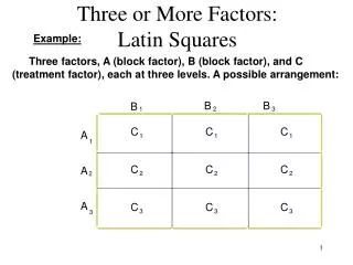
Three or More Factors: Latin Squares. Example:. Three factors, A (block factor), B (block factor), and C (treatment factor), each at three levels. A possible arrangement:. B. B. B. 1. 2. 3. C. C. C. A. 1. 1. 1. 1. C. C. C. A. 2. 2. 2. 2. A. C. C. C. 3. 3. 3. 3.

Three or More Factors: Latin Squares
E N D
Presentation Transcript
Three or More Factors: Latin Squares Example: Three factors, A (block factor), B (block factor), and C (treatment factor), each at three levels. A possible arrangement: B B B 1 2 3 C C C A 1 1 1 1 C C C A 2 2 2 2 A C C C 3 3 3 3
Notice, first, that these designs are squares; all factors are at the same number of levels, though there is no restriction on the nature of the levels themselves. Notice, that these squares are balanced: each letter (level) appears the same number of times; this insures unbiased estimates of main effects. How to do it in a square? Each treatment appears once in every column and row. Notice, that these designs are incomplete; of the 27 possible combinations of three factors each at three levels, we use only 9.
Example: Three factors, A (block factor), B (block factor), and C (treatment factor), each at three levels, in a Latin Square design; nine combinations. B B B 1 2 3 C C C A 1 2 3 1 C C C A 2 3 1 2 A C C C 3 1 2 3
B B B B 1 2 3 4 C C C C A 4 3 2 1 1 8 5 5 8 7 7 8 9 0 9 9 7 C C C C A 1 2 3 4 2 9 6 2 8 1 7 8 4 5 7 7 6 C C C C A 3 4 1 2 3 8 4 8 8 4 1 7 8 4 7 7 6 C C C C A 2 1 4 3 4 8 3 1 9 5 2 8 0 6 8 7 1 Example with 4 Levels per Factor FACTORS VARIABLE Lifetime of a tire (days) Automobiles A four levels Tire positions B four levels Tire treatments C four levels
r t g and each at m levels Three factors , , , The Model for (Unreplicated) Latin Squares Example: m i = 1,... y 1, m ... = + + + + j = , ijk j k ijk i ... , k m Y = A + B + C + e = 1, AB, AC, BC, ABC Note that interaction is not present in the model. Same three assumptions: normality, constant variances, and randomness.
Putting in Estimates: = y + ( y – y ) + ( y – y ) + ( y – y ) + R y ijk ... i .. ... . j . ... .. k ... or bringing y••• to the left – hand side , ( y – y ) = ( y – y ) + ( y – y ) + ( y – y ) + R , ijk ... i .. ... . j . ... .. k ... Variability among yields associated with Rows Variability among yields associated with Columns Variability among yields associated with Inside Factor Total variability among yields = + + y – y – y – y + 2 y where R = ijk i .. . j . .. k ...
Actually, R = y - y - y - y + 2 y ... ijk i .. . j . .. k = ( y - y ) ( y - y ) - ijk ... i .. ... y y ) - - ( . j . ... - ( y - y ), .. k ... An “interaction-like” term. (After all, there’s no replication!)
The analysis of variance (omitting the mean squares, which are the ratios of second to third entries), and expectations of mean squares: S o u r c e o f S u m o f D e g r e e s o f E x p e c t e d v a r i a t i o n s q u a r e s f r e e d o m v a l u e o f m e a n s q u a r e m R o w s m – 1 + V 2 m ( y – y ) 2 Rows i .. ... i = 1 m C o l u m n s m – 1 + V 2 m ( y – y ) 2 Col . j . ... j = 1 m I n s i d e m – 1 + V 2 m ( y – y ) 2 Inside factor .. k ... f a c t o r k = 1 b y s u b t r a c t i o n ( m – 1)( m – 2) 2 Error T o t a l m – 1 2 2 ( y – y ) ijk ... i j k
The expected values of the mean squares immediately suggest the F ratios appropriate for testing null hypotheses on rows, columns and inside factor.
Our Example: (Inside factor = Tire Treatment) Tire Position Auto.
General Linear Model: Lifetime versus Auto, Postn, TrtmntFactor Type Levels Values Auto fixed 4 1 2 3 4Postn fixed 4 1 2 3 4Trtmnt fixed 4 1 2 3 4Analysis of Variance for Lifetime, using Adjusted SS for TestsSource DF Seq SS Adj SS Adj MS F PAuto 3 17567 17567 5856 2.17 0.192Postn 3 4679 4679 1560 0.58 0.650Trtmnt 3 26722 26722 8907 3.31 0.099Error 6 16165 16165 2694Total 15 65132 Unusual Observations for LifetimeObs Lifetime Fit SE Fit Residual St Resid 11 784.000 851.250 41.034 -67.250 -2.12R
SPSS/Minitab DATA ENTRYVAR1 VAR2 VAR3 VAR4855 1 1 4962 2 1 1848 3 1 3831 4 1 2877 1 2 3817 2 2 2. . . .. . . .. . . .871 4 4 3
Latin Square with REPLICATION • Case One: using the same rows and columns for all Latin squares. • Case Two: using different rows and columns for different Latin squares. • Case Three: using the same rows but different columns for different Latin squares.
Treatment Assignments for n Replications • Case One: repeat the same Latin square n times. • Case Two: randomly select one Latin square for each replication. • Case Three: randomly select one Latin square for each replication.
Example: n = 2, m = 4, trtmnt = A,B,C,D Case One: • Row = 4 tire positions; column = 4 cars
Case Two • Row = clinics; column = patients; letter = drugs for flu
Case Three • Row = 4 tire positions; column = 8 cars
ANOVA for Case 1SSBR, SSBC, SSBIF are computed the same way as before, except that the multiplier of (say for rows) m (Yi..-Y…)2 becomes mn (Yi..-Y…)2and degrees of freedom for error becomes(nm2 - 1) - 3(m - 1) = nm2 - 3m + 2
ANOVA for other cases: • SS: please refer to the book, Statistical Principles of research Design and Analysis by R. Kuehl. • DF: # of levels – 1 for all terms except error. DF of error = total DF – the sum of the rest DF’s. Using Minitab in the same way can give Anova tables for all cases.
Graeco-Latin Squares In an unreplicated m x m Latin square there are m2 yields and m2 - 1 degrees of freedom for the total sum of squares around the grand mean. As each studied factor has m levels and, therefore, m-1 degrees of freedom, the maximum number of factors which can be accommodated, allowing no degree of freedom for factors not studied, is A design accommodating the maximum number of factors is called a complete Graeco-Latin square: m – 1 2 = m + 1 m – 1
In an unreplicated complete Graeco-Latin square all degrees of freedom are used up by factors studied. Thus, no estimate of the effect of factors not studied is possible, and analysis of variance cannot be completed.
But, consider incomplete Graeco-Latin Squares: b1 b2 b3 b4 b5 c4d4 c5d5 a1 c1d1 c2d2 c3d3 c2d3 a2 c3d4 c4d5 c5d1 c1d2 c3d5 a3 c4d1 c5d2 c1d3 c2d4 c5d3 a4 c1d4 c2d5 c3d1 c4d2 c5d4 c1d5 c2d1 c3d2 c4d3 a5
We test 4 different Hypotheses. ANOVA TABLE df SSQ SOURCE 4 4 4 4 8 A B C D Error SSBA SSBB SSBC SSBD SSW • • • • • by Subtraction TSS 24