IMPORT TARIFFS AND QUOTAS UNDER PERFECT COMPETITION
850 likes | 2.24k Vues
8. 1 A Brief History of the World Trade Organization 2 The Gains from Trade 3 Import Tariffs for a Small Country 4 Import Tariffs for a Large Country 5 Import Quotas 6 Conclusions. IMPORT TARIFFS AND QUOTAS UNDER PERFECT COMPETITION. Introduction.

IMPORT TARIFFS AND QUOTAS UNDER PERFECT COMPETITION
E N D
Presentation Transcript
8 1 A Brief History of the World Trade Organization 2 The Gains from Trade 3 Import Tariffs for a Small Country 4 Import Tariffs for a Large Country 5 Import Quotas 6 Conclusions IMPORT TARIFFS AND QUOTAS UNDER PERFECT COMPETITION
Introduction • During the 2000 presidential campaign, President George W. Bush promised to consider implementing a tariff on the imports of steel. • This was a political move to secure votes in large steel-producing states as the tariffs would “protect” the domestic producers of steel. • The steel tariff is an example of a trade policy—a government action meant to influence the amount of international trade. © 2008 Worth Publishers ▪ International Economics ▪ Feenstra/Taylor
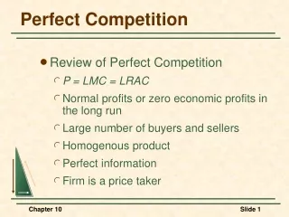
Introduction • Because gains from trade are unevenly spread, producers often feel the government should help them limit losses due to competition from trade. • Trade policy can include the use of import tariffs (taxes on imports), import quotas (limits on imports), and subsidies for exports. • We will assume that firms are perfectly competitive. They produce a homogeneous good and are small compared to the market. • Firms are price takers © 2008 Worth Publishers ▪ International Economics ▪ Feenstra/Taylor
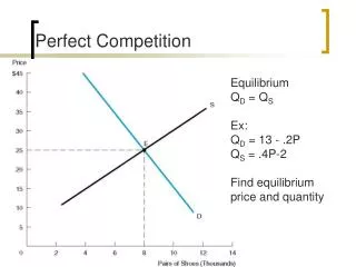
The Gains from Trade • We will now demonstrate the gains from trade using Home demand and supply curves, together with the concepts of consumer surplus and producer surplus. • Consumer and Producer Surplus • Figure 8.1 (a) shows the Home demand curve D where consumers face a price of P1. • Remember, CS is the difference between the price the consumer is willing to pay and the actual price. • Part (b) of figure 8.1 illustrates producer surplus. • Remember that PS is the difference between MC and price, where the supply curve represents a firm’s MC. © 2008 Worth Publishers ▪ International Economics ▪ Feenstra/Taylor
The Gains from Trade Total Consumer surplus, CS Surplus for consumer purchasing quantity D2 Figure 8.1 (a) Adding up all the individual surplus for each point on the demand curve gives us total consumer surplus—the area between the demand and the price paid—up to the quantity sold The demand curve gives us the consumer’s value for each unit of the good. Given P1, consumers will buy a total of D1. A consumer who purchases D2 has a value of P2, but only has to pay P1 – that gives surplus equal to (P2-P1) Price P2 P1 D D2 D1 Quantity © 2008 Worth Publishers ▪ International Economics ▪ Feenstra/Taylor
The Gains from Trade Total Producer surplus, PS Surplus for firm producing quantity S0 Figure 8.1 (b) The supply curve gives us the consumer’s value for each unit of the good. Given P1, producers will sell a total of S1. A producer who sells S0 has a MC of P0, but gets P1. That gives surplus equal to (P1-P0) Adding up all the individual surpluses for each point on the supply curve gives us total producer surplus—the area between the supply and the price received—up to the quantity sold. Price S P1 P0 S0 S1 Quantity © 2008 Worth Publishers ▪ International Economics ▪ Feenstra/Taylor
The Gains from Trade CS PS • No trade equilibrium • Again we consider the world of two countries, Home and Foreign, with producers and consumers. • Total Home welfare can be measured by adding up consumer and producer surplus. • We will compare the welfare in Home in no-trade and free-trade situations. Figure 8.2 Price No-trade equilibrium S A PA D Q0 Quantity © 2008 Worth Publishers ▪ International Economics ▪ Feenstra/Taylor
The Gains from Trade • Free Trade for a Small Country • Suppose Home can now engage in trade. • The world price PW is determined by the supply and demand in the world market (shown in in figure 8.2 (b)). • Suppose Home is a small country. • Price taker in the world market • Faces a fixed price at PW • Assume PW is below the Home no-trade price PA. • At the lower price,Home will be an importer of the product at the world price. © 2008 Worth Publishers ▪ International Economics ▪ Feenstra/Taylor
The Gains from Trade Imports, M1 Figure 8.2 At lower world price, consumer surplus increases to a+b+d an increase of b+d from no-trade (b) Free Trade Price At lower world price, producer surplus falls to c a decrease of b from no-trade S a PA PW b Gain in trade is triangle d with area equal to ½(M1)(PA-PW) d c D S1 D1 Quantity © 2008 Worth Publishers ▪ International Economics ▪ Feenstra/Taylor
The Gains from Trade • Home Import Demand Curve • We can derive the import demand curve, shown in figure 8.3 • The relationship between the world price of a good and the quantity of imports demanded by Home consumers. • At the no-trade equilibrium, there are zero imports • This is shown as point A′ in panel (b). • At the world price of PW, the quantity demanded is greater than quantity supplied, and we import M1. • This is point B in panel (b). • Joining A′ and B gives import demand curve M. © 2008 Worth Publishers ▪ International Economics ▪ Feenstra/Taylor
The Gains from Trade Figure 8.3 (b) (a) No-trade equilibrium Each point on the import demand curve is a point that corresponds to Home imports at a given Home price Price Price S A' PA PW A B Import demand curve, M D M1 Imports S1 Q0 D1 Quantity Imports, M1 © 2008 Worth Publishers ▪ International Economics ▪ Feenstra/Taylor
Import Tariffs for a Small Country • Free Trade for a Small Country • Since Home is a small country, the tariff does not affect world prices. • The Foreign export supply curve X* is horizontal at the world price PW. • Effect of the Tariff • The new export supply curve shifts up to X*+t. • Quantity demanded falls while quantity supplied rises • However, as firms increase the quantity produced, the marginal costs of production rise. • The domestic price will equal the import price. © 2008 Worth Publishers ▪ International Economics ▪ Feenstra/Taylor
Import Tariffs for a Small Country Home price rises by the amount of the tariff. Home supply increases and Home demand decreases Imports fall to M2 C PW+t X*+t M2 S2 D2 M2 Figure 8.4 No-trade equilibrium Price Price S A B Foreign export supply, X* PW D M M1 Imports Quantity S1 D1 © 2008 Worth Publishers ▪ International Economics ▪ Feenstra/Taylor
Import Tariffs for a Small Country • Effect of the Tariff on Consumer Surplus • With the tariff, consumers now pay the higher price, PW+t, and their surplus is the area under the demand curve and above the higher price, PW+t. • The fall in consumer surplus due to the tariff is the area in-between the two prices and to the left of Home demand, (a+b+c+d) in panel (a.1) of figure 8.5. • This area is the amount that consumers lose due to the higher price caused by the tariff. © 2008 Worth Publishers ▪ International Economics ▪ Feenstra/Taylor
Import Tariffs for a Small Country b d a c Figure 8.5 (a.1) No-trade equilibrium Lost consumer surplus due to the higher price with the tariff is equal to the shaded area (a+b+c+d) Price S A PW+t PW D S1 S2 D2 D1 Quantity M2 © 2008 Worth Publishers ▪ International Economics ▪ Feenstra/Taylor
Import Tariffs for a Small Country • Effect of the Tariff on Producer Surplus • With the tariff, producer surplus is the area above the supply and below the higher price, PW+t. • Since the tariff increases Home price, firms can sell more goods, and producer surplus increases • This area, a in figure 8.5 (a.2), is the amount that Home firms gain due to the higher price caused by the tariff. • Increases in producer surplus can benefit Home workers but at the expense of consumers. © 2008 Worth Publishers ▪ International Economics ▪ Feenstra/Taylor
Import Tariffs for a Small Country Figure 8.5 (a.2) No-trade equilibrium The gain in producer surplus due to the higher price with the tariff is equal to the shaded area (a) Price S A b d PW+t PW a c D S1 S2 D2 D1 Quantity M2 © 2008 Worth Publishers ▪ International Economics ▪ Feenstra/Taylor
Import Tariffs for a Small Country • Effect of the Tariff on Government Revenue • In addition to the tariff’s impact on consumers and producers, it also affects government revenue. • The amount of revenue collected is the tariff t times the quantity of imports (D2 – S2). • In figure 8.5 panel (a.3), the revenue is shown by area c. • The collection of revenue is a gain for the government in the importing country. © 2008 Worth Publishers ▪ International Economics ▪ Feenstra/Taylor
Import Tariffs for a Small Country Figure 8.5 (a.3) The gain in government revenue due to the tariff is equal to the shaded area (c) This equals the tariff, t, times the quantity of imports, M2 No-trade equilibrium Price S A b d PW+t PW a c D S1 S2 D2 D1 Quantity M2 © 2008 Worth Publishers ▪ International Economics ▪ Feenstra/Taylor
Import Tariffs for a Small Country • Overall Effect of the Tariff on Welfare • Note, we do not care whether the consumers facing higher prices are rich or poor, and do not care whether the specific factors in the industry earn a lot or a little. • The overall impact of the tariff in the small country can be summarized as follows: Fall in consumer surplus -(a+b+c+d) Rise in producer surplus +a Rise in government revenue +c Net effect on Home welfare -(b+d) • The areas b and d in figure 8.5 (a) correspond to the triangle (b+d) in figure 8.5 (b) and is the net welfare loss. • We refer to this area as a deadweight loss—it is not offset by a gain elsewhere in the economy. © 2008 Worth Publishers ▪ International Economics ▪ Feenstra/Taylor
Import Tariffs for a Small Country Figure 8.5 (a) The deadweight loss is the loss to Home that is not offset by a corresponding gain No-trade equilibrium Price S a is a transfer from consumers to producers c is a transfer from consumers to government (b+d) is deadweight loss—losses not offset by other gains b = production distortion d = consumption distortion A b d PW+t PW a c D S1 S2 D2 D1 Quantity M2 © 2008 Worth Publishers ▪ International Economics ▪ Feenstra/Taylor
Import Tariffs for a Small Country Price X*+ t X* M Imports M2 M1 Figure 8.5 (b) Dead weight loss due to tariff, b+d C © 2008 Worth Publishers ▪ International Economics ▪ Feenstra/Taylor
Why are Tariffs Used? • Why do so many countries use tariffs if they always lead to deadweight losses? • One idea is that developing countries do not have any other source of revenue. • Import tariffs are “easy-to-collect” relative to income taxes. • However, to the extent that developing countries recognize that tariffs have a higher deadweight loss, we would expect that over time they will shift away from such “easy-to-collect” taxes. • A second reason is politics. • The might government care more about producer surplus than consumer surplus. • The benefits to producers (and their workers) are typically more concentrated on specific firms and states than the costs to consumers, which are spread nationwide. © 2008 Worth Publishers ▪ International Economics ▪ Feenstra/Taylor
U.S. Tariffs on Steel • We will estimate the deadweight loss due to the U.S. steel tariff in place from March 2002 to December 2003. • President Bush requested that the U.S. International Trade Commission (ITC) initiate a Section 201 investigation into the steel industry. • The tariffs varied across products, ranging from 10 to 20%—shown in Table 8.1—then falling over time to be eliminated after 3 years. 2008 Worth Publishers ▪ International Economics ▪ Feenstra/Taylor
U.S. Tariffs on Steel • President Bush took the recommendation of the ITC but applied even higher tariffs, ranging from 8% to 30%. • Knowing the U.S. trading partners would be upset by this, President Bush exempted some countries from the tariffs. • These included Canada, Mexico, Jordan, and Israel, which all have free trade agreements with the U.S., and 100 small developing countries that were exporting only a very small amount of steel to the U.S. 2008 Worth Publishers ▪ International Economics ▪ Feenstra/Taylor
U.S. Tariffs on Steel Table 8.1 2008 Worth Publishers ▪ International Economics ▪ Feenstra/Taylor
U.S. Tariffs on Steel • Deadweight Loss due to the Steel Tariff • We need to estimate the areas of triangle b+d we found in figure 8.5(b). • The base is the change in imports, ΔM, and the height is the increase in domestic price, ΔP = t. • Deadweight loss then equals DWL = ½ t ΔM. • It is convenient to measure the deadweight loss relative to the value of imports, which is PW*M. • We will also use the percentage tariff, t/PW, and the percentage change in the quantity of imports, % ΔM = ΔM/M. 2008 Worth Publishers ▪ International Economics ▪ Feenstra/Taylor
U.S. Tariffs on Steel Figure 8.5 (b) We can measure DWL with the area of the triangle b+d from figure 8.5 (b) DWL = ½ t ΔM Price Deadweight loss due to the tariff, b+d PW+t t c PW M M2 M1 Imports ΔM 2008 Worth Publishers ▪ International Economics ▪ Feenstra/Taylor
U.S. Tariffs on Steel • Using these definitions, the deadweight loss relative to the value of imports can be rewritten as: • The most commonly used products had a tariff of 30%, so the percentage increase in the price is t/PW = 0.3, leading to %ΔM = 0.3. 2008 Worth Publishers ▪ International Economics ▪ Feenstra/Taylor
U.S. Tariffs on Steel • This leads to a DWL of • The value of steel imports affected by the tariff was about $4.7 billion prior to March 2002 and $3.5 billion after March 2002. • Average imports over the two years were $4.1 billion. • The dollar magnitude of deadweight loss is equal to $185 million. 2008 Worth Publishers ▪ International Economics ▪ Feenstra/Taylor
Import Tariffs for a Large Country • Under the small country assumption that we have used so far, the importing country is always harmed due to the tariff. • The small country is a world price taker. • If we consider a large enough importing country or a large country, however, then we might expect that its tariff will change the world price. • Its imports are large enough that it can affect world price with a change in its imports. © 2008 Worth Publishers ▪ International Economics ▪ Feenstra/Taylor
Import Tariffs for a Large Country • Foreign Export Supply • If the Home country is large, then the Foreign export supply curve X* is no longer horizontal at the world price PW. • We construct the Foreign export supply curve in a fashion similar to the import demand curve. • In panel (a) of figure 8.6, we show the Foreign demand curve D* and supply curve S*, giving price of PA* at A*. • At this point, Foreign exports are zero. Suppose the world price is PW above PA*. • At the higher price, there is a Foreign excess supply of X1* = S1* - D1*, which will be exported at the price of PW at point B*. © 2008 Worth Publishers ▪ International Economics ▪ Feenstra/Taylor
Import Tariffs for a Large Country Foreign export supply, X* B* PW PA* A*' A* S1* D1* X1* Foreign exports, X1* Figure 8.6 (b) World Mkt (a) Foreign Mkt World price increases to PW, increasing exports to X1* This gives us our Foreign export supply curve for the large country Price Price At the world price, PA*, exports are zero at A*’ S* D* Home import demand, M Exports Quantity © 2008 Worth Publishers ▪ International Economics ▪ Feenstra/Taylor
Import Tariffs for a Large Country • Effect of the Tariff • Figure 8.7 we show the effect when Home applies a tariff of t dollars on imports. • Foreign export supply curve shifts up by exactly the amount of the tariff, shifting from X* to X*+t. • The Home price rises by less than t, and the Foreign producers receive, P*, which is less than PW. • The tariff drives a wedge between what Home consumers pay and what foreign producers receive, with the difference, t, going to the Home government. © 2008 Worth Publishers ▪ International Economics ▪ Feenstra/Taylor
Import Tariffs for a Large Country Figure 8.7 (without welfare effects) (a) Home market (b) Foreign market Price Price No-trade equilibrium X*+t S A X* t C P*+t t t PW B* P* C* D M Imports M2 M1 S1 S2 D2 D1 Quantity M2 M1 © 2008 Worth Publishers ▪ International Economics ▪ Feenstra/Taylor
Import Tariffs for a Large Country • Home Welfare Fall in consumer surplus -(a+b+c+d) Rise in producer surplus +a Rise in government revenue +(c + e) Net effect on Home welfare e – (b+d) + (e) • The triangle (b+d) is the deadweight loss due to the tariff. • Area e offsets part of the loss. • If e > (b+d), then Home is better off. • If e < (b+d), then Home is worse off. © 2008 Worth Publishers ▪ International Economics ▪ Feenstra/Taylor
Import Tariffs for a Large Country Figure 8.7 (with welfare effects) If the gain of e is greater than the loss of (b+d), Home gains (a) Home market (b) Foreign market No-trade equilibrium Price Price X*+t S b+d t X* A C P*+t PW P* a c b d B* C* e e D M S1 S2 D2 D1 Quantity M2 M1 Imports © 2008 Worth Publishers ▪ International Economics ▪ Feenstra/Taylor
Import Tariffs for a Large Country • Home welfare may improve, but it comes at the expense of foreign exporters. • Foreign and World Welfare • The Foreign loss, measured by (e+f) also in figure 8.7, is the loss in Foreign producer surplus from selling fewer goods to Home at a lower price. • The area e is the terms-of-trade gain for Home (P*<PW) but an equivalent terms-of-tradeloss for Foreign. • Additionally, there is an extra deadweight loss in Foreign of f, giving a combined total greater than the benefits to Home. • Therefore, it is sometimes called the “beggar thy neighbor” tariff. • There is a world welfare loss = b + d + f © 2008 Worth Publishers ▪ International Economics ▪ Feenstra/Taylor
Import Tariffs for a Large Country Figure 8.7 (with welfare effects) Foreign loses (e+f) as loss of Foreign producer surplus, from selling fewer goods at a lower price (a) Home market (b) Foreign market No-trade equilibrium Price Price X*+t S b+d t X* A C P*+t PW P* a c b d B* f e e C* D M S1 S2 D2 D1 Quantity M2 M1 Imports © 2008 Worth Publishers ▪ International Economics ▪ Feenstra/Taylor
U.S. Tariffs on Steel Once Again • Optimal Tariff • Compute the deadweight loss (area b+d) and the terms-of-trade gain (area e) for each imported steel product. • Rather than do all these calculations, however, we can use the concept of the optimal tariff. • The tariff that leads to the maximum increase in welfare for the importing country. • We have shown that for a small tariff, a large country can gain. But if the tariff is too large, the country will still lose. • Figure 8.8 graphs Home welfare against the level of the tariff. 2008 Worth Publishers ▪ International Economics ▪ Feenstra/Taylor
U.S. Tariffs on Steel Once Again The Optimal tariff maximizes the Importer’s welfare, Point C Figure 8.8 Too high of a tariff will decrease importer’s welfare and can increase to the point where there is no trade Terms of trade gain exceeds deadweight loss Importer’s Welfare Terms of trade gain is less than deadweight loss C B' Free Trade B A No Trade Tariff Optimal Tariff Prohibitive Tariff 2008 Worth Publishers ▪ International Economics ▪ Feenstra/Taylor
U.S. Tariffs on Steel Once Again • Optimal Tariff Formula • The optimal tariff depends on the elasticity of Foreign export supply, EX*. • Optimal Tariff Formula Optimal Tariff = 1/EX*. • For a small importing country, the elasticity of Foreign export supply is infinite, and so the optimal tariff is zero. • As the elasticity of Foreign export supply decreases, Foreign export supply curve is steeper, the optimal tariff is higher. 2008 Worth Publishers ▪ International Economics ▪ Feenstra/Taylor
U.S. Tariffs on Steel Once Again • Optimal Tariffs for Steel • If we apply this formula to the U.S. steel tariffs, we can see how the tariffs applied compare to the theoretical optimal tariff. • Table 8.2 shows various steel products along with their respective elasticities of export supply to the U.S. • We can compare the actual tariff to the optimal tariff to see where there were gains and where there were losses from the tariffs. • But what about retaliation?... 2008 Worth Publishers ▪ International Economics ▪ Feenstra/Taylor
U.S. Tariffs on Steel Once Again Table 8.2 2008 Worth Publishers ▪ International Economics ▪ Feenstra/Taylor
Import Quotas • On January 1, 2005, China was poised to become the world’s largest exporter of textiles and apparel. • On that date, the Multifibre Arrangement (MFA) was abolished. • Under the MFA, import quotas restricted the amount of nearly every textile and apparel product that was imported to Canada, Europe, and the U.S. • The quotas were to protect their own domestic firms producing those products. • The threat of import competition from China led the U.S. and Europe to negotiate new quotas with China. © 2008 Worth Publishers ▪ International Economics ▪ Feenstra/Taylor
Import Quotas • Import Quota in a Small Country • Suppose the import quota of M2<M1 is imposed. • This essentially gives us a vertical supply curve, X in panel b (at prices above PW). • Fixes the import quantity at M2, price rises to P2. • Qty supplied rises to S2 and qty demanded falls to D2. • For every level of import quota, there is an equivalent import tariff • Has the same price and quantity effects as the quota. • The equivalent tariff is: t = P2 – PW © 2008 Worth Publishers ▪ International Economics ▪ Feenstra/Taylor
Import Quotas d b C b+d P2 a c c D2 S2 M2 Figure 8.9 (with quota) Consumers loses surplus of (a+b+c+d), producers gain (a). Welfare of Home depends on what happens to (c), the total quota rents. At the new higher price P2, Home Supply increases to S2, Demand decreases to D2 and imports fall to M2 The new Export Supply curve crosses the Import Demand curve at a new price and quantity of imports With the Quota, the Foreign export supply becomes vertical at the quota quantity Always have a deadweight loss of (b+d) like the tariff No-trade equilibrium S Price Price A Foreign export supply, X* B PW Home import demand, M D Quantity D1 Imports S1 M1 (b) Import market (a) Home market © 2008 Worth Publishers ▪ International Economics ▪ Feenstra/Taylor
Import Quotas • There are four possible ways these rents can be allocated. • Giving the Quota to Home Firms: • Quota licenses can be given to Home firms • Permits to import the quantity allowed under the quota system. • The net effects on Home welfare due to the quota are then as follows: Fall in consumer surplus -(a+b+c+d) Rise in producer surplus +a Quota rents earned at Home +c Net effect on Home welfare: -(b+d) • This is the same loss we saw with a tariff. • (b+d) is still a deadweight loss associated with the quota. © 2008 Worth Publishers ▪ International Economics ▪ Feenstra/Taylor
Import Quotas • Rent Seeking • Because of the gains associated with owning a quota license, firms have an incentive to engage in inefficient activities in order to obtain them. • How licenses are allocated matters. • If licenses are allocated in proportion to each firm’s production, Home firms will likely produce more than they can sell just to obtain the import licenses for the following year. • Firms might engage in bribery or other lobbying activities to obtain the licenses. © 2008 Worth Publishers ▪ International Economics ▪ Feenstra/Taylor
Import Quotas • Some suggest that the waste of resources devoted to rent seeking could be as large as the value of the rents themselves, c. • If rent seeking occurs, welfare loss of quota is: Fall in consumer surplus -(a+b+c+d) Rise in producer surplus +a Net effect on Home welfare: -(b+c+d) • This loss is larger than a tariff. • It is thought rent seeking is worse in developing countries. © 2008 Worth Publishers ▪ International Economics ▪ Feenstra/Taylor