Post-processing analysis of climate simulation data using Python and MPI
Post-processing analysis of climate simulation data using Python and MPI. John Dennis ( dennis@ucar.edu ) Dave Brown ( dbrown@ucar.edu ) Kevin Paul ( kpaul@ucar.edu ) Sheri Mickelson ( mickelso@ucar.edu ). Motivation.

Post-processing analysis of climate simulation data using Python and MPI
E N D
Presentation Transcript
Post-processing analysis of climate simulation data using Python and MPI John Dennis (dennis@ucar.edu) Dave Brown (dbrown@ucar.edu) Kevin Paul (kpaul@ucar.edu) Sheri Mickelson (mickelso@ucar.edu)
Motivation • Post-processing consumes a surprisingly large fraction of simulation time for high-resolution runs • Post-processing analysis is not typically parallelized • Can we parallelize post-processing using existing software? • Python • MPI • pyNGL: python interface to NCL graphics • pyNIO: python interface to NCL I/O library
Consider a “piece” of CESM post-processing workflow • Conversion of time-slice to time-series • Time-slice • Generated by the CESM component model • All variables for a particular time-slice in one file • Time-series • Form used for some post-processing and CMIP • Single variables over a range of model time • Single most expensive post-processing step for CMIP5 submission
The experiment: • Convert 10-years of monthly time-slice files into time-series files • Different methods: • Netcdf Operators (NCO) • NCAR Command Language (NCL) • Python using pyNIO (NCL I/O library) • Climate Data Operators (CDO) • ncReshaper-prototype (Fortran + PIO)
Duration: Serial NCO 5 hours 14 hours!
Approaches to Parallelism • Data-parallelism: • Divide single variable across multiple ranks • Parallelism used by large simulation codes: CESM, WRF, etc • Approach used by ncReshaper-prototype code • Task-parallelism: • Divide independent tasks across multiple ranks • Climate models output large number of different variables • T, U, V, W, PS, etc.. • Approach used by python + MPI code
Single source Python approach • Create dictionary which describes which tasks need to be performed • Partition dictionary across MPI ranks • Utility module ‘parUtils.py’ only difference between parallel and serial execution
Example python code import parUtils as par … rank = par.GetRank() # construct global dictionary ‘varsTimeseries’ for all variables varsTimeseries = ConstructDict() … # Partition dictionary into local piece lvars = par.Partition(varsTimeseries) # Iterate over all variables assigned to MPI rank for k,v in lvars.iteritems(): ….
Throughput: Parallel methods(4 nodes, 16 cores) data-parallelism task-parallelism
Duration: NCO versus pyNIO + MPI w/compression 7.9x (3 nodes) 35x speedup (13 nodes)
Conclusions • Large amounts of “easy-parallelism” present in post-processing operations • Single source python scripts can be written to achieve task-parallel execution • Factors of 8 – 35x speedup is possible • Need ability to exploit both task and data parallelism • Exploring broader use within CESM workflow Expose entire NCL capability to python?