Download

1 / 33
330 likes | 473 Vues
Committees of hydrological models specialized on high and low flows. 1 UNESCO-IHE Institute for Water Education , Delft ,The Netherlands 2 Delft University of Technology, The Netherlands 3 Russian State Hydrometeorological University. Dimitri Solomatine 1,2 (presenting)

E N D
Committees of hydrological models specialized on high and low flows 1 UNESCO-IHE Institute for Water Education , Delft ,The Netherlands 2 Delft University of Technology, The Netherlands 3 Russian State Hydrometeorological University Dimitri Solomatine1,2(presenting) and NagendraKayastha1 VadimKuzmin3
Motivation • Theory of modelling: • Complex systems (processes) are comprised of multiple components (simpler sub-processes) • Simple models often cannot adequately reflect complexity • Idea: • instead of one, use several specialised models, each representing such a sub-process (hydrometeorological situation) • Optimize the way they are combined • This may allow for better response in changing conditions Solomatine and Kayastha : Committee models, IAHS, Gothenburg, 2013
Outline Committee modelling: examples and experiences Building specialized models Fuzzy committee of specialized models Case studies: Leaf catchment, USA Lissbro, Sweden Results and conclusions Ideas for future work Solomatine and Kayastha : Committee models, IAHS, Gothenburg, 2013
Combination of models (committees, ensembles, modular models): earlier work • Shamseldin, A. Y., K. M. O'Connor and G. C. Liang (1997). Methods for combining the outputs of different rainfall–runoff models. J. Hydrol. 197(1–4): 203-229. • Xiong, L., Shamseldin, A. Y. and O’Connor, K. M. (2001). A nonlinear combination of the forecasts of rainfall-runoff models by the first-order Takagi-Sugeno fuzzy system, J. Hydrol., 245(1), 196–217. • Abrahart, R. J. and See, L. M. (2002). Multi-model data fusion for river flow forecasting: an evaluation of six alternative methods based on two contrasting catchments, Hydrol. Earth Syst. Sci., 6, 655–670. • Solomatine, D. P. and Siek, M. (2006). Modular learning models in forecasting natural phenomena, Neural Networks, 19, 215–224. • Oudin L., Andréassian V., Mathevet T., Perrin C. & Michel C.,(2006), Dynamic averaging of rainfall-runoff model simulations from complementary model parameterization. Water Resources Research, 42. • G. Corzo and D.P. Solomatine (2007). Baseflow separation techniques for modular ANN modelling in flow forecasting. Hydrol. Sci. J., 52(3), 491-507. • Fenicia, F., Solomatine, D. P., Savenije, H. H. G. and Matgen, P. Soft combination of local models in a multi-objective framework. HESS, 11, 1797-1809, 2007. • Toth E. (2009). Classification of hydro-meteorological conditions and multiple artificial neural networks for streamflow forecasting, HESS, 13, 1555–1566. • Kayastha N., Ye J., Fenicia F., Solomatine D.P. (2013). Fuzzy committees of specialised rainfall-runoff models: further enhancements, HESSD, 10, 675-697, doi:10.5194/hessd-10-675-2013. Solomatine and Kayastha : Committee models, IAHS, Gothenburg, 2013
Limitations of “single model” approach Complexity of the hydrological processes The simplicity of the “conceptual” modelling paradigm often leads to errors in representing all the different complexity of the physical processes in the catchment A single model often cannot capture the full variability of the system response varying order of magnitude in flow value variance of error dependent on flow value A single aggregate measure criteria of model performance is traditionally used Divide and conquer… Small is beautiful… Solomatine and Kayastha : Committee models, IAHS, Gothenburg, 2013
Steps in building a committee of RR models Identification of specialized models, e.g.: “soft separation” scheme to identify “low flows” and “high flows” (Fenicia et al., 2007) baseflow separation (Corzo and Solomatine, 2006) identifying rising and falling limbs (Jain and Shrinivasulu, 2006) separation by threshold value of flow (Willems, 2009) Transformation of flow (Oudin et al. 2006) Objective functions (errors) definition Calibration of specialised models (Multi-objective, Single objective) Models combination (committees, ensembles, averaging) Check performances Solomatine and Kayastha : Committee models, IAHS, Gothenburg, 2013
Modular models for modelling sub-processes D.P. Solomatine (2006). Optimal modularization of learning models in forecasting environmental variables. iEMSs 3rd Biennial Meeting: Summit on Environmental Modelling and Software (A. Voinov, A. Jakeman, A. Rizzoli, eds.) Solomatine & Xue. (2004) M5 model trees compared to neural networks: application to flood forecasting in the upper reach of the Huai River in China. ASCE J. Hydrologic Engineering, 9(6), 491-501. … Papers by Shamseldin et al.,1997; Abrahart & See 2002; Jain et al., 2006; Oudin et al., 2006; etc. Complex process Sub-process1 Sub-process2 Sub-process K • Splitting into sub-processes: • Domain experts (humans) specify such processes • Computational intelligence algorithms discover “hidden” processes based on observed data • Combination of both approaches Solomatine and Kayastha : Committee models, IAHS, Gothenburg, 2013
Modular models: Methods of data splitting G. Corzo and D.P. Solomatine. (2007) Baseflow separation techniques for modular artificial neural network modelling in flow forecasting. Hydrological Sciences J., 52(3), 491-507. • Using machine learning methods to group (cluster) data corresponding to different hydrometerological regimes: • k-means, Fuzzy c-means • Self-organising maps • Applying hydrological knowledge for flow separation: • Tracer-based methods • Threshold-based flow separation • Constant-slope method for baseflow separation • Recursive filter for baseflow separation Solomatine and Kayastha : Committee models, IAHS, Gothenburg, 2013
Modular models using clustering • Modular Models are built for each cluster of data K-means cluster (Bagmati training data set) Qt+1 (forecast discharge) P (current precipitation) Q (current discharge) Solomatine and Kayastha : Committee models, IAHS, Gothenburg, 2013
Optimal model structure using recursive filter for baseflow separation G. Corzo and D.P. Solomatine (2007). Knowledge-based modularization and global optimization of ANN models in hydrologic forecasting. Neural Networks, 20, 528–536 Ekhardt 2005 Parameter BFImax=0.5 (Chapman and Maxwell 1996) Parameter a= 0.99 (Recession coefficient ) Parameter a=0.01 (Recession coefficient) Solomatine and Kayastha : Committee models, IAHS, Gothenburg, 2013
Performance of the Modular Model using recursive filter vs Single (global) model Bagmati catchment Solomatine and Kayastha : Committee models, IAHS, Gothenburg, 2013
Committee models States- based dynamic averaging i) Soil moisture accounting (Oudin et al., 2006) ii) Other states: quick and slow flows Inputs-based dynamic averaging Outputs-based dynamic averaging i) Fuzzy committee (Fenicia et al., 2007, Kayastha et al., 2013) ii) Weights based on observed and simulated flows A B C 12 Solomatine and Kayastha : Committee models, IAHS, Gothenburg, 2013
Specialized models Fenicia, F., Solomatine, D. P., Savenije, H. H. G. and Matgen, P. Soft combination of local models in a multi-objective framework. HESS, 11, 1797-1809, 2007. • Error on low flows • Error on high flows By applying weighting factors to the model residuals Two models are built – for low and high flows Each objective functions (wRMSE) weights flows differently Solomatine and Kayastha : Committee models, IAHS, Gothenburg, 2013
Fuzzy committee of specialised models (1) Low-flow model QLF R, E Combiner (fuzzy committee) Qc High-flow model QHF For this range of flow both models work The membership functions are subject to the accurate optimization of the parameters (γ, δ), Solomatine and Kayastha : Committee models, IAHS, Gothenburg, 2013
Fuzzy committee of specialised models (2) Kayastha, Ye, Fenicia, Solomatine. (2013) Fuzzy committees of specialised rainfall-runoff models: further enhancements, HESSD, 10, 675-697, doi:10.5194/hessd-10-675-2013 • Further enhancements (2012-2013): optimization all parameters of - • weighted schemes and • fuzzy membership functions • Experiments conducted on calibration data, and model verification on test data • Tested optimization algorithms • Multi- objective – NSGA II (Deb, 2001) • Single objective: Genetic algorithm – GA (Goldberg, 1989), Adaptive cluster covering – ACCO (Solomatine, 1999) • Tested on three case studies • Alzette, Bagmati and Leaf catchment Solomatine and Kayastha : Committee models, IAHS, Gothenburg, 2013
Fuzzy committee of specialised models (3) Cont. Kayastha et al. , (2013) • Influenceof different weighting schemes used in objective functions for calibration of high and low flow models: • Quadratic, N=2 • Cubic, N=3 Solomatine and Kayastha : Committee models, IAHS, Gothenburg, 2013
Fuzzy committee of specialised models (4) Cont. Kayastha et al., (2013) • The shape of membership functions are subjected to the parameters (γ, δ), which switch the flow regimes (between low flow and high flow). Solomatine and Kayastha : Committee models, IAHS, Gothenburg, 2013
Case study : Leaf catchment Area - 1924 km2 , 10 years of daily data , 6 yrs calibration / 4 yrs verification One of the identified Pareto-optimal front corresponding to model parameterisations using weighting scheme to separate flow regimes and the objective function value in calibration and verification periods Calibration Verification Solomatine and Kayastha : Committee models, IAHS, Gothenburg, 2013
Current study: Lissbro, Sweden (1) Lissbrocatcment , 97.0 km², Sweden, 17 years of daily data HBV model (13 parameters) was used Optimization algorithm used for calibration: Adaptive cluster covering – ACCO (Solomatine, 1995, 1999) All experiments are conducted on calibration data, and verified on test data Complete period: 01/01/1984 - 31/12/2010 Calibration periods: P1: 01/01/1984 - 31/12/1988 P2: 01/01/1989 - 31/12/1993 P3: 01/01/1994 - 31/12/1998 P4: 01/01/1999 - 31/12/2003 P5: 01/01/2006 - 31/12/2010 Solomatine and Kayastha : Committee models, IAHS, Gothenburg, 2013
Current study: Lissbro, Sweden (2) Statistical properties of data Solomatine and Kayastha : Committee models, IAHS, Gothenburg, 2013
Conceptual model: HBV Conceptual lumped model 3 tanks 13 parameters to calibrate Solomatine and Kayastha : Committee models, IAHS, Gothenburg, 2013
Objective functions used Nash and Sutcliffe Efficiency (NSE) Root mean squared error (RMSE) Log transformed flows (Oudin et al. 2006) Weighted RMSE on high flows (Fenicia et al. 2007) Weighted RMSE on low flows (Fenicia et al. 2007) 22 Solomatine and Kayastha : Committee models, IAHS, Gothenburg, 2013
Experiment -1: Level 2: single model, calibration on 5 subsets Single model performance (NSE) over the 5 pre-defined periods) Means of 5 performances 23 Solomatine and Kayastha : Committee models, IAHS, Gothenburg, 2013
Experiment-1: Comparing committee models to the single one A) State-based dynamic averaging (Oudin et al., 2006) B) Output-based dynamic averaging using fuzzy committee (Fenicia et al., 2007 ; Kayastha et al., 2013) C) Output-based dynamic averaging using observed flows Solomatine and Kayastha : Committee models, IAHS, Gothenburg, 2013
Experiment-2: single model, calibration on 1+2+3 Model performance (NSE) over the 2 pre-defined periods Calibration period – Periods 1 + 2 + 3 Verification period – Periods 4 + 5 P1: 01/01/1984 - 31/12/1988 P2: 01/01/1989 - 31/12/1993 P3: 01/01/1994 - 31/12/1998 P4: 01/01/1999 - 31/12/2003 P5: 01/01/2006 - 31/12/2010 In verification Committees are better than the single models 25 Solomatine and Kayastha : Committee models, IAHS, Gothenburg, 2013
Experiment -2: fragments of hydrograph The fragments of hydrograph (Experiment -2) 26 Solomatine and Kayastha : Committee models, IAHS, Gothenburg, 2013
Model errors for various years: the committee model is more robust Single model vs Committee model (Fuzzy) lower SD for Committee model Yearly NSE Yearly NSE low flow Yearly Bias (Qsim/Qobs) 27 Solomatine and Kayastha : Committee models, IAHS, Gothenburg, 2013
Model errors for different periods: the committee model is more robust Single model vs Committee model (Fuzzy) lower SD in Committee model NSE 28 Solomatine and Kayastha : Committee models, IAHS, Gothenburg, 2013
Conclusions (1) Splitting of data into small subsets does not allow for committee models to become significantly better than a single model However using larger sets (P1+P2+P3) for calibration, makes committee models more accurate than a single model Mean of NSE Lowe r than single param. model Solomatine and Kayastha : Committee models, IAHS, Gothenburg, 2013
Conclusions (2) Committees of specialized models can be used when an overall model fails to identify triggers and thresholds in the catchment behavior is seen as a natural way of introducing additional complexity and hence adaptivity Committee models were initially developed for improving accuracy of short-term forecasts, and they do it well. However our hypothesis is: inherent capacity of committee models to react to short-term changes in hydrometeorologic condition may provide the mechanism for capturing the long-term changes as well Solomatine and Kayastha : Committee models, IAHS, Gothenburg, 2013
Further work Defining what is a “hydrometeorological regime” at different time scales To try to deal with non-stationarity by using non-stationary parameters (and machine-learning them) Developing more adaptive dynamic combination schemes able to deal with the long term changes in regimes “Philosophical questions” to think about: When several models are combined the notion of “state” seem to disappear – is it a problem? Some combination schemes are not conservative , i.e. may generate or loose water (“violates physics”) - is it bad ? We calibrate models knowing data is bad (especially for peaks) – is it right ? Solomatine and Kayastha : Committee models, IAHS, Gothenburg, 2013
Welcome to our COURSES on Flood Risk Management (July, 3 weeks) New data sources for flood modelling (September, 1 week) KULTURisk Summer School Flood risk reduction: perception, communication, governance Delft (The Netherlands) 9-12 September 2013 Erasmus MundusFlood Risk Management Masters 2013-2015 www.FloodRiskMaster.org Solomatine and Kayastha : Committee models, IAHS, Gothenburg, 2013
Thank you very much! Solomatine and Kayastha : Committee models, IAHS, Gothenburg, 2013