Download
1 / 44
440 likes | 585 Vues
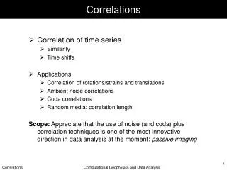
Correlations (part I). Mechanistic/biophysical plane: - What is the impact of correlations on the output rate, CV, ...

E N D
Mechanistic/biophysical plane: • - What is the impact of correlations on the output rate, CV, ... • Bernarder et al ‘94, Murphy & Fetz ‘94, Shadlen & Newsome ’98, Stevens & Zador ’98, Burkit & Clark ’99, Feng & Brown ‘00, Salinas & Sejnowski ’00, Rudolf & Destexhe ’01, Moreno et al ’02, Fellows et al ‘02 , Kuhn et al ’03, de la Rocha ’05 • - How are correlations generated? Timescale? • Shadlen & Newsome ’98, Brody ’99, Svirkis & Rinzel ’00, Tiensinga et al ’04, Moreno & Parga, • 2. Systems level: • - do correlations participate in the encoding of information? • Shadlen & Newsome ’98, Singer & Gray ’95, Dan et al ’98, Panzeri et al ’00, DeCharms & Merzenich ’95, Meister et al, Neimberg & Latham ‘00 • - linked to behavior? • Vaadia et al, ’95, Fries et al ’01, Steinmetz et al ’00, …
Type of correlations: stimulus s response: r1, r2, ... , rn 1.- Noise correlations: 2.- Signal correlations:
Quantifying spike correlations trial index t1i,r t2i,r t3i,r ... cell index 1. Stationary case: • Corrected cross-correlogram:
Quantifying spike correlations 2. Non-stationary case: • Joint Peristimulus time-histogram: • Time averaged cross-correlogram:
Quantifying spike correlations • Correlation coefficient: • Spike count: if T >>
How to generate artificial correlations? 1. Thinning a “mother” train. “mother” train (rate R) deletion rate = p * R
How to generate artificial input correlations? 2. Thinning a “mother” train (with different probs.) “mother” train (rate R) deletion rate = p * R rate = q * R
How to generate artificial inputcorrelations? 3. Thinning & jittering a “mother” train “mother” train (rate R) deletion + jitter rate = p * R random delay: exp(-t/tc) / tc
How to generate artificial inputcorrelations? 4. Adding a “common” train “common” train (rate R) summation rate = r + R
How to generate artificial inputcorrelations?: 5. Gaussian input Diffusion approximation 1
1 2 How to generate artificial inputcorrelations?: 5. Gaussian input White input:
Impact of correlations on the input current of a single cell: Excitation Rate = nE 1 2 … NE Poisson inputs; Zero-lag synchrony 1 2 … NI Inhibition Rate = nI
Impact of correlations on the output rate: Balanced state Unbalanced state
The development of correlations: a minimal model. 1. Morphological common inputs.
The development of correlations: a minimal model. 2. Afferent correlations
The development of correlations: a minimal model. 3. Connectivity
Development of correlations: common inputs Shadlen & Newsome ‘98
Development of correlations: common inputs & synaptic failures R(1-x) Rp(1-x) p p Rx Rp2x+Rpx(1-p) p R(1-x) Rp(1-x) p • Independent: Rp(1-x)+Rpx(1-p)= Rp(1-xp)= Reff (1-xeff) • Common: Rp2x = Reff xeff • where we have defined: • Effective rate: Reff = R p • Effective overlap: xeff = x p
Development of correlations: common inputs & synaptic failures
Development of correlations: common inputs. Experimental data.
Biophysical constraints of how fast neurons can synchronize their spiking activity • Rubén Moreno Bote • Nestor Parga, Jaime de la Rocha and Hide Cateau
Outline • I. Introduction. • II. Rapid responses to changes in the input variance. • III. How fastcorrelations can be transmitted? • Biophysical constrains. Goals: 1. To show that simple neuron models predict responses of real neurons. 2. To stress the fact that “qualitative”, non-trivial predictions can be made using mathematical models without solving them.
I. Introduction.Temporal changes in correlation Vaadia el al, 1995 deCharms and Merzenich, 1996
I. Temporal modulations of the input. mean variance Diffusion approximation: white noise process with mean zero and unit variance
I. Temporal modulations of the input. common variance
I. Problems Problem 1: How fast a change in mand scan be transmitted? Leaky Integrate-and-Fire (LIF) neuron Problem 2: How fast two neurons can synchronize each other? common source of noise
II. Probability density function and the FPE Description of the density P(V,t) with the FPE P(V) P(threshold)=0 V q Firing rate:
II. Non-stationary response. Fast responses predicted by the FPE P(V,t) P(threshold, t)=0 V q Mean input current 1. Firing rate response time Variance of the current 2. Firing rate response time Described by the equation
II. Rapid response to instantaneous changes of s (validity for more general inputs) Change in input variance Change in the input correlations for dif. correlation statistics Silberberg et al, 2004 Change in the mean Moreno et al, PRL, 2002.
II. Stationary rate as a function of tc >0 =0 <0 Moreno et al, PRL, 2002.
III. Correlation between a pair of neurons Cross-correlation function = P( t1 , t2 ) time lag = t1 - t2 0 Moreno-Bote and Parga, submitted
III. Transient synchronization responses. Exact expression for the cross-corr. The join probability density of having spikes at t1 and t2 for IF neurons 1 and 2 receiving independent and common sources of white noise is: Total input variances at indicated times for neurons 1 and 2. Joint probability density of the potentials of neurons 1 and 2 at indicated times
III. Predictions • Increasing any input variance produces an “instantaneous” increase • of the synchronization in the firing of the two neurons. • 2. If the common variance increases and the independent variances • decrease in such a way that the total variance remains constant, the • neurons slowly synchronize. • 3. If the independent variances increase, there is a sudden increase in the • synchronization, and then it reduces to a lower level. … biophysical constraints that any neuron should obey!!
III. Slow synchronization when the total variances does not change.
III. Fast synchronization to an increase of common variance.
III. Fast synchronization to an increase of independent variance, and its slow reduction.