Download
1 / 19
190 likes | 210 Vues
Learn how to make quantitative predictions of hydraulic properties of different media using Miller's comprehensive methodology for geometric similarity. Understand the necessary conditions and mathematical equations for scaling pressure, conductivity, and time. Examples and data from laboratory studies provided.

E N D
Miller Similarity and Scaling of Capillary Properties How to get the most out of your lab dollar by cheating with physics
A little orientation... • How can we take information about the hydraulic properties of one media to make quantitative predictions of the properties of another media? • 1956 Miller and Miller presented a comprehensive methodology. • Bounds on our expectations: • can’t expect to make measurements in a sand and hope to learn about the behavior of clays: • fundamentally differing in their chemical properties and pore-scale geometric configuration. • To extrapolate from one media to another, the two systems must be similar in the geometric sense (akin to similar triangles).
Characterizing each medium • We need “characteristic microscopic length scales” of each media with a consistent definition. • Need ’s in some dimension which can be identified readily and reflects the typical dimensions at the grain scale. • In practice people often use the d50 as their as it is easy to measure and therefore widely reported. • Any other measure would be fine so long as you are consistent in using the same measure for each of the media.
Enough generalities, let’s see how this works! • Assumptions Need For Similarity: • Media: Uniform with regard to position, orientation and time (homogeneous, isotropic and permanent). • Liquid: Uniform, constant surface tension, contact angle, viscosity and density. Contact angle must be the same in the two systems, although surface tension and viscosity may differ. • Gas: Move freely in comparison to the liquid phase, and is assumed to be at a uniform pressure. • Connectivity: Funicular states in both the air and water: no isolated bubbles or droplets. • What about hysteresis? No problem, usual bookkeeping.
Rigorous definition of geometric similarity • Necessary and sufficient conditions: • Medium 1 and 2 are similar if, and only if, there exists a constant = 1/2 such that if all length dimensions in medium 1 are multiplied by , the probability of any given geometric shape to be seen in the scaled medium1 and medium 2 are identical. • Most convenient to define a “scaled medium” which can then be compared to any other similar medium. • Scaled quantity noted with dot suffix: K• is scaled conductivity.
Getting to some math.. • Consider Pressure of two media with geometrically similar emplacement of water. • Volumetric moisture content will be the same in the two systems. • For any particular gas/liquid interface Laplace’s equation gives the pressure in terms of the reduced radius Rwhere is the contact angle, is the surface tension, and p is the difference in pressure between the gas and liquid.
Multiplying both sides by • Stuff on left side is the same for any similar media, • THUS • Stuff on the right side must be constant as well. • We have a method for scaling the pressure!
Example Application • Let’s calculate the pressure in medium 1 at some moisture content given that we know the pressure in medium 2 at . From above, we note that the pressures are related simply asso we may obtain the pressure of the second media as
Some data from our lab • Scaling of the characteristic curves for four similar sands. Sizes indicated by mesh. Schroth, M.H., S.J. Ahearn, J.S. Selker and J.D. Istok. Characterization of Miller-Similar Silica Sands for Laboratory Hydrologic Studies. Soil Sci. Soc. Am. J., 60: 1331-1339, 1996.
How about scaling hydraulic conductivity • Need to go back to the underlying physical equations to derive the correct expression for scaling. • Identify the terms which make up K in Darcy’s law in the Navier-Stokes equation for creeping flow • Compared to Darcy’s law • which can be written
Equating, and Solving for K we findThe velocity is at the pore-scale, so we see that • where l is a unit of length along pore-scale flow. Nowso equation [2.131] may be rewritten asPutting the unscaled variables on the left we see that
From last slide: • The right-hand side of [2.135] is only dependent on the properties of the scaled media, implying that the left-hand side must be as well Careful: p is not the scaled pressure! Should writeThe scaling relationship for permeability!
Example • Two similar media at moisture content : Scaled conductivities will be identical or, solving for K2 in terms of K1 we find which can also be written in terms of pressure (ψ)
Last scaling parameter required: time • By looking to the macroscopic properties of the system, we can obtain the scaling relationship for time • Consider Darcy’s law and the conservation of mass. • In the absence of gravity Darcy’s law states • Multiplying both sides by , we find
Scaling time... • From a macroscopic viewpoint, both v and are functions of the macroscopic length scale, say L. The product L is the reduced form of the gradient operator. So we can multiply both sides by L to put the right side of this equation in the reduced formSince right side is, then left side is in reduced form, thus the reduced macroscopic velocity is given by
Finishing up t scaling • Would like to obtain the scaling parameter for time, say , such that t = t•. Using the definition of velocity we can write and using the fact that x•=x/L and t•=t, v• can be rewritten • Now solving for we find • and solving for t• • JOB DONE!!
Squared • scaling of K • w.r.t. • particle size
Data from Warrick • et al. demonstrating • scaling of • saturation - • permeability • relationship
Warrick et al. • demonstration • of scaled • pressure - • saturation • relationship