Download
1 / 64
640 likes | 775 Vues
Contribution to: II EULAG WORKSHOP SOPOT, POLAND, SEPTEMBER, 13-16, 2010. IMPLEMENTATION OF SURFACE ENERGY BALANCE FLUXES INTO EULAG MODEL: MADRID CASE STUDY R. San José, J. L. Pérez, J.L. Morant 1 and R.M. González 2 1 Environmental Software and Modelling Group

E N D
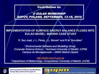
Contribution to: II EULAG WORKSHOP SOPOT, POLAND, SEPTEMBER, 13-16, 2010 IMPLEMENTATION OF SURFACE ENERGY BALANCE FLUXES INTO EULAG MODEL: MADRID CASE STUDY R. San José, J. L. Pérez, J.L. Morant1 and R.M. González2 1Environmental Software and Modelling Group Computer Science School – Technical University of Madrid (UPM) Campus de Montegancedo – 28660 Madrid (Spain) http://artico.lma.fi.upm.es 2Department of Meteorology, Complutense University of Madrid (UCM)
WRF/NOAH/UCM output with 0.2 km spatial resolution as BC’s and IC’s will be used for EULAG model simulations with 4 m spatial resolution . Different runs have been done in three cities (Madrid (Spain), Florence (Italy) and Gliwice (Poland) over a 1 km x 1 km model domain. • Surface energy fluxes have been implemented into EULAG code based on the procedures applied in UCM and NOAH/Land-surface model. • A new micro shadow model SHAMO has been developed to calculate shadow areas (including reflections in urban areas) and short wave radiation in high resolution (meters) domains .
MODELS: WRF WRF : Next generation mesoscale meteorological model. The equation set is fully compressible, Eulerian and nonhydrostatic. It is conservative for scalar variables. The model uses terrain-following, hydrostatic-pressure vertical coordinate with the top of the model being a constant pressure surface. The horizontal grid is the Arakawa-C grid. The time integration scheme in the model uses the third-order Runge-Kutta scheme, and the spatial discretization employs 2nd to 6th order schemes (Skamarock, W.C., Klemp, J.B., Dudhia, J., Gill, D.O., Barker, D.M., Wang, W., Powers, J.G., 2005. A description of the advanced research WRF version 2, NCAR Technical Note. National Center for Atmospheric Research, Boulder, CONCAR/TN-468+STR, 100pp. )
MODELS. WRF (ARW) WRF : Weather Research and Forecasting modeling system. http://www.mmm.ucar.edu/wrf/users
WRF/NOAH/UCM • Physics Options used in WRF: • Cumulus Parameterization: • GRELL-DEVENYI ENSEMBLE SCHEME (Grell, G. A., and D. Devenyi, 2002: A generalized approach to parameterizing convection combining ensemble and data assimilation techniques. Geophys. Res. Lett., 29(14), Article 1693. ) • PBL Scheme and Diffusion: • Yonsei University (YSU) PBL (Hong, S.-Y., Dudhia, J., 2003. Testing of a new non-local boundary layer vertical diffusion scheme in numerical weather prediction applications. In: Proceedings of the 16th Conference on Numerical Weather Prediction, Seattle, WA. ) • Explicit Moisture Scheme : • LIN et al.SCHEME microphysics (Lin, Y.L., R. D. Farley, and H. D. Orville, 1983: Bulk parameterization of the snow field in a cloud model. J. Appl. Meteor., 22, 1065-1092 )
WRF/NOAH/UCM • Physics Options used in WRF: • Radiation Schemes: • Rapid Radiative Transfer Model (RRTM) longwave radiation(E.J. Mlawer, S.J. Taubman, P.D. Brown, M.J. Iacono and S.A. Clough, Radiative transfer for inhomogeneous atmospheres: RRTM, a validated correlated-k model for the longwave, J. Geophys. Res. 102 (D14) (1997), pp. 16663–16682 ) • Simple cloud-interactive shortwave radiation schemeDudhia radiation ( Dudhia, Numerical study of convection observed during the winter monsoon experiment using a mesoscale two-dimensional Model, J. Atmos. Sci.46 (1989), pp. 3077–3107)
WRF/NOAH/UCM Land surface model: NOAH/UCM (Chen, F., Kusaka, H., Tewari, M., Bao, J.-W., Kirakuchi, H., 2004. Utilizing the coupled WRF/LSM/Urban modeling system with detailed urban classification to simulate the urban heat island phenomena over the greater Houston area. In: Proceedings of the 5th Conference on Urban Environment, 22–26 August 2004, Vancouver, BC, Canada.)
DOMAINS. MOTHER DOMAIN Lambert Conformal Conic (-3.703, 40.412) 119*119 grid cells 16.2 km. resolution Lowert left corner (-963900, -963900) Iberian Peninsula
DOMAINS. 1 LEVEL NESTED DOMAIN Lambert Conformal Conic (-3.703, 40.412) 117*117 grid cells 1.8 km. resolution Lowert left corner (-105300, --105300) Madrid Community
DOMAINS. 2 LEVEL NESTED DOMAIN Lambert Conformal Conic (-3.703, 40.412) 127*127 grid cells 0.2 km. resolution Lowert left corner (-13500, --13500) Madrid Municipality
MESOSCALE DOMAINS. WRF ARCHITECTURE MOTHER DOMAIN 59*59 grid cells 48.6 km. resolution Lower left corner (-1433700, -1433700) DT:300 s. Projection: Lambert Conformal Conic LEVEL 1: 37*37 grid cells 5.4 km. resolution Lower left corner (-121500, -121500) DT: 30 s. LEVEL 2: 28*28 grid cells 0.2 km. resolution Lower left corner (-2700, -2700) DT: 0.6 s. • Global model data: GFS • One way nesting. (two-way nesting uses higher CPU time in this case)
MODELS. WRF-NOAH-UCM The UCM (Urban Canopy Model) is a single layer model, used to consider the effects of urban geometry on surface energy balance and wind shear for urban regions (H. Kusaka and F. Kimura, Coupling a single-layer urban canopy model with a simple atmospheric model: impact on urban heat island simulation for an idealized case, Journal of Applied Meteorology 43 (2004), pp. 1899–1910. ) To better represent the physical processes involved in the exchange of heat, momentum, and water vapor in the mesoscale model, the Urban Canopy Model (UCM ) is coupled to the WRF model (Tewari, M., Chen, F., Kusaka, H.,2006. Implementation and evaluation of a single-layer urban model in WRF/Noah. In: Proceedings of the 7th WRF Users’ Workshop, June 2006)
MODELS: WRF-NOAH-UCM • UCM: Take the urban geometry into account in its surface energy budgets and wind shear calculations. Radiative, thermal, moisture effects and canopy flow model are accounted for in the UCM. • Main issues: • - 2-D street canyons that are parameterized to represent the effects of urban geometry on urban canyon heat distribution • Shadowing from buildings and reflection of radiation in the canopy layer • 3D Radiation treatment. Canyon orientation and diurnal cycle of solar azimuth angle • Wind profile within the urban canopy layer (Swaid 1993)
MODELS: WRF-NOAH-UCM • Main issues: • Multi-layer roof, wall and road models. • Anthropogenic heat flux • Sensible heat fluxes are calculated from Jurge´s formula (Tanaka 1993) plus Monin-Obukhow similarity theory over urban canopy (Masson 2000 TEB). • - Surface temperatures are determined from the multilayer heat equation solved numerically • - Roof and road surfaces are impermeable layers. • UCM can be run on-line/ off-line mode.
WRF/NOAH/UCM. HIGHT RESOLUTION INPUT DATA USGS+ 3 UCM CATEGORIES (31,32,33) FROM CLC 2000 (250 m) with 0.2 KM RES. TERRAIN HEIGHT 0.2 KM RES.
Urban Building Height Urban Street Width Urban Roof Width WRF/NOAH/UCM. HIGH RESOLUTION INPUT DATA
18:00 GMT DAILY AVG DAILY MAX WRF/NOAH/UCM. OUTPUTS Air Temperature 2M (k) 28/06/2008
WRF/NOAH/UCM. VALIDATION Air Temperature 2M
MESOSCALE TO URBAN SCALE WRF/NOAH/UCM 200 m. RES WIND COMPONENTS POTENTIAL TEMPERATURE TURBULENCE KINETIC ENERGY INITIAL & BOUNDARY CONDITIONS CFD/EULAG 4 m. RES
WRF HIGH RESOLUTION Temperature & Winds CFD EULAG MODULE MICRO FLUXES MODULE MICRO SHADOW MODULE Sensible heat Flux Short wave radiation CFD EULAG – UCM/NOAH MICRO FLUXES- SHADOW MODEL T_eulag_new = T_eulag + (SHF / Rhoo*cpp*CHS) SHF: Sensible heat flux. Rhoo: Air density. CPP=1004. CHS=Surface exchange coefficient f (Wrf)
MICROSYS-EULAG URBAN SIMULATIONS TIME PERIOD: 28/06/2008 07:00 - 12:00 – 18:00 – 21:00 TIME STEP: 0.01 (7200 time steps) OUTPUT FREQUENCY: 10 s. EULAG OPTIONS: - Numerical approximation: Eulerian conservation law - Method to represent the edifice-> Immersed boundary (R. Mittal and G. Iaccarino, Immersed boundary methods, Ann. Rev. Fluid Mech. 37 (2005), pp. 239–261. ) - Turbulence model Smagorinsky Smagorinsky, J., 1993, ‘‘Some Historical Remarks on the Use of Nonlinear Viscosities,’’ Large Eddy Simulation of Complex Engineering and Geophysical Flows, Cambridge University Press, Cambridge, UK, pp. 3–36. - Moist and simple ice model: ON
SETUP MICROSYS-EULAG MADRID 250*250 grid cells 4 m. resolution Height 100 m MADRID BUILDINGS 2D & 3D VIEW Global mapper
MICROSYS-EULAG URBAN SIMULATIONS. RESULTS POTENTIAL TEMPERATURE (K) MADRID 28/06/2008 6 Min. Surface & Vertical planes YZ, XZ
WRF – MICROSYS (EULAG+NOAH/UCM) • RADIATION FORCING: • Long wave • Short ware • ATMOSPHERIC FORCING: • Pressure • Humidity • Precipitation PBL SCHEME SURFACE SCHEME : Surface exchange coefficient for vertical turbulent exchange (Monin-Obukov theory) Wind & Temperature from CFD (EULAG) LAND SURFACE SCHEME: NOAH/UCM High resolution 4m.
Implementation of urban flux estimations into EULAG (MICROSYS)
Implementation of urban flux estimation into EULAG (MICROSYS)
Implementation of urban flux estimation into EULAG (MICROSYS): SIMPLE SHADOW MODEL • Simple shadow model using ideal canyons in order to calculate short wave radiation (SWR) by each grid cell (4 meters) SWR = SWRi + SWRr i: Incident short wave radiation r: Reflected short wave radiation Each grid cell is associated to the closet building to get the “h” parameter. Data used: City 3d Building GIS w: Street width h: Building height ls: Shadow length
Implementation of urban flux estimation into EULAG (MICROSYS): SIMPLE SHADOW MODEL Shadow length: ls ls = h * tan σz * sin σn σz : Solar zenit angle (from WRF radiation model) σn : Street orientation (from GIS data) IF ls > w THEN ls =w (Shadow length <= Street width) Short wave radiation from WRF is splited into direct(d) & diffuse(q): SWRd = SWR_WRF * 0.8 SWRq = SWR_WRF * 0.2
Implementation of urban flux estimation into EULAG (MICROSYS): SIMPLE SHADOW MODEL SWRi : Incident short wave radiation SWRr : Reflected short wave radiation α : Ground Albedo αw : Wall Albedo FSKY = 1 - Fwalltoground FSKY : Sky view factor Fwalltoground : Wall view factor
Implementation of NON urban flux estimation into EULAG (MICROSYS): NOAH/LAND-SURFACE MODEL • GROUND HEAT FLUX (GH) • GH= DF ( T – STC(1) ) / DSOIL • DF: Thermal diffusivity • T : skin temperature • STC(1) : soil temperature (firs layer) • DSOIL: width layer soil • THERMAL DIFFUSIVITY (DF) • SATURATED THERMAL CONDUCTIVITY • DRY THERMAL CONDUCTIVITY • TOTAL SOIL MOISTURE CONTENT • POROSITY • QUARTZ CONTENT
Implementation of NON urban flux estimation into EULAG (MICROSYS): NOAH/LAND-SURFACE MODEL • SENSIBLE HEAT FLUX (SH) • SH= (CH * CP *SFCPRS) / (R * T2V) * (TH2 – T) • CH : Surface exchange coefficient (surface scheme) • SFCPRS : Surface pressure • T2V : Virtual temperature (from cfd) • TH2: Potential temperature (from cfd) • CP,R: Constants • LATENT HEAT FLUX (LH) • LH = EDIR + EC + ETT • EC : Canopy water evaporation • EDIR: Direct soil evaporation • ETT : Total plant transpiration
Implementation of NON urban flux estimation into EULAG (MICROSYS) • POTENTIAL EVAPORATION ETP SPLITTING • EDIR = “SOIL MOISTURE CONTENT (SMC)” * ETP • EC = “CANOPY MOISTURE CONTENT (CMC) ” * ETP • CMC = CMC_old + (RAIN – EC) • ETT = “PLANT COEFFICIENT” * ETP • PLANT COEFFICIENT CANOPY RESISTANCE - LAI: leaf area index – Rc_min ≈ f(vegetation type) – F1 ≈ f(amount of PAR:solar insolation) – F2 ≈ f(air temperature: heat stress) – F3 ≈ f(air humidity: dry air stress) – F4 ≈ f(soil moisture: dry soil stress)
Implementation of NON urban flux estimation into EULAG (MICROSYS) • POTENTIAL EVAPORATION ETP (PENMAN) • Potential evaporation: amount of evaporation that would occur if a sufficient water source were available. Surface and air temperature, insolation, and wind all affect this • ETP = EPSCA * RCH / 2.501e+6 • EPSCA = (A * RR + RAD * DELTA) / (DELTA + RR) • RCH = (SFCPRS / (287.4*T2V)) * 1004.5 * CH • A SATURATION SPECIFIC HUMIDITY & 2M SPECIFIC HUMIDITY • RR = [ EMISSIVITY * T4 * 6.48e-8 / (SFCPRS * CH) + 1.0 ] + “RAIN” • RAD = (TR – EMISSIVITY * T4 * T – GH ) / RCH*TH2-SFCTMP • DELTA Slope of saturation specific humidity curve at T = surface temperature (SFCTMP) • CH : Surface exchange coefficient (surface model)
Implementation of NON urban flux estimation into EULAG (MICROSYS) • SURFACE WATER BALANCE • dSCM = P - R – ETP • dSMC = change in soil moisture content (SMC) • P = precipitation • R = runoff (Rainfall infiltration rate Schaake & Koren model. Calculations based on hydraulic conductivity and diffusivity ) • ETP = Potential evaporation • (P-R) = infiltration
MICROSYS LATENT HEAT FLUX: (LH) • 1. NO URBAN CELLS • LH = LH_NATURAL (CALCULATED BY NOAH) • LH_NATURAL = ETP (IF ETP < 0) • LH_NATURAL = EDIR + EC + ETT (IF ETP>0) • 2. URBAN CELLS • LH=LH_URB (CALCULATED BY UCM) + (1-FRC_URB) * LH_NATURAL (CALCULATED BY NOAH) LH: Latent Heat Flux (w/m2) ETP: Potential evaporation (w/m2) EDIR: Direct soil evaporation (w/m2) EC: Canopy Water evaporation (w/m2) ETT: Total Plant Transpiration (w/m2) FRC_URB: Urban Fraction
MICROSYS-MADRID- DETAILED LANDUSES AIRBONEDATA 4m RES LANDUSE 1: water (lake) 2: water 3: trees 4: green grass 5: bright bare 6:dark bare 7: roads 8: other pavement 9: asphalt roofs 10: tile roofs 11:concrete roofs 12: metal roofs 13: shadows 14: no data 1KM * 1KM
MICROSYS-MADRID-DETAILED LANDUSES AIRBONE >>> USGS NOAH 4m RES LANDUSE USGS (AIRBONE) 1: urban (7-14 airbone) 7: grassland (4 airbone) 15: mixed forest (3 airbone) 16: water (1,2 airbone) 19: barren (5,6 airbone) 1KM * 1KM
MICROSYS-FLUXES (SIMPLE SHADOW MODEL). MADRID 28/06/2008 12:01
MICRO-URBAN SOLAR RADIATION MODEL • Multiple reflections • -non idealized canyon street approach • - Direct and diffuse solar radiation are calculated with clouds effects Direct Solar Radiation Diffuse Solar Radiation Reflections Shadows
MICRO-URBAN SOLAR RADIATION MODEL 3D Building GIS Sun location Downward short radiation Mesoscale Radiation Model (WRF-Dudhia) Sun location (xyz) Shadows Sky view factor Direct & Diffuse Reflections Micro-Urban Radiation Model SHAMO (UPM) Global solar radiation (each cell) (short) LAND SURFACE SCHEME: NOAH/UCM High resolution
MICRO-URBAN SOLAR RADIATION MODEL Final Solar Radiation: (Including m reflections) FSRi,m = ∑k FSRk,m-1 * ALB * FREFLECTION FSRi,m : Final Solar Radiation, grid cell i, after m reflections FSRk,m-1 : Final Solar Radiation, grid cell j, after m-1 reflections ALB : Surface Albedo FREFLECTION : Reflection Factor m=0 Initial Solar Radiation ISR (No reflections yet) Iterative calculations STOP Reflections Increase FSR < 1% ISR
MICRO-URBAN SOLAR RADIATION MODEL Initial Solar Radiation: (No reflections) ISR = FSHADOW * DIRSR + FSKY *DIFSR FSHADOW: Building shadow effect. FSHADOW=1 The grid cell is in the sun FSHADOW=0 The grid cell is in the shade DIRSR: Direct Solar Radiation (W/m2) DIFSR: Diffuse Solar Radiation (W/m2) FSKY: Sky View Factor [0-1]
FSHADOW=1 FSHADOW=0 MICRO-URBAN SOLAR RADIATION MODEL. SHADOWS FSHADOW: - 3D Straight line from center of the grid cell to the sun - Follow the straight line, if it collides with a building grid cell then FSHADOW=0 else FSHADOW=1
MICRO-URBAN SOLAR RADIATION MODEL. SHADOWS SUN´s POSITON: - Inputa data from mesoscale radiation model: * Declination angle (d) * Zenith angle (z) * Hour angle (w) - Celestial coordinate system: * Solar altitude angle (α): 90º - z * Solar azimuth angle (y):
MICRO-URBAN SOLAR RADIATION MODEL. SHADOWS SUN´s POSITON:
MICRO-URBAN SOLAR RADIATION MODEL. SHADOWS SUN´s POSITON: Cartesian coordinates x = r cos(α) sin (y) y = r cos(α) cos(y) z = r sin(α) R: Sphere radius covering the 3d domain X-axis. East-West direction Y-axis. North-South direction (0,0,0) Center of the grid cell
MICRO-URBAN SOLAR RADIATION MODEL. SHADOWS SUN MADRID SHADOWS 1km*1km domain 4m resolution grid cells White areas = buildings NO SUN
MICRO-URBAN SOLAR RADIATION MODEL. SKY VIEW FACTOR FSKY & FREFLECTION: - 3D RAY TRACKING METHOD - CASTING RAYS FROM A HEMISPHERE LOCATED ON THE CENTER OF EACH GRID CELL - FINAL POINT OF EACH RAY: X= k cos(σ) Y=k sin(σ) Z= (r2 – k2) ^(1/2) - COUNT NUMBER OF RAYS THAT COLLIDE WITH BUILDING GRID CELL - MINIMUM NUMBER OF RAYS 35000 IN A 1KM*1KM DOMAIN σ: Ray direction angle [0,180º] k : Ray Height [0,r]
MICRO-URBAN SOLAR RADIATION MODEL. SKY VIEW FACTOR FSKY & FREFLECTION: - FREFLECTION: FRACTION OF RAYS THAT COLLIDE WITH BUILDINGS GRID CELLS IS THE CORRESPONDING REFLECTION FACTOR. - FSKY: (1 – FREFLECTION) , RAYS ARE NOT REFLECTED. THIS IS THE SKY VIEW FACTOR - High computing DEMAND -> PARALLEL APPROACH MADRID DOMAIN: 1000*1000*100 meters 4m resolution: * 34752 RAYS 1 CPU 95 Min. * 34752 RAYS 50 CPUs 2.40 Min. * 135014 RAYS 50 CPUs 6.50 Min.