2.4 Describing Distributions Numerically
2.4 Describing Distributions Numerically. Numerical and More Graphical Methods to Describe Univariate Data. 2 characteristics of a data set to measure. center measures where the “middle” of the data is located variability measures how “spread out” the data is.

2.4 Describing Distributions Numerically
E N D
Presentation Transcript
2.4 Describing Distributions Numerically Numerical and More Graphical Methods to Describe Univariate Data
2 characteristics of a data set to measure • center measures where the “middle” of the data is located • variability measures how “spread out” the data is
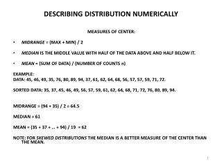
The median: a measure of center Given a set of n measurements arranged in order of magnitude, Median= middle value n odd mean of 2 middle values, n even • Ex. 2, 4, 6, 8, 10; n=5; median=6 • Ex. 2, 4, 6, 8; n=4; median=(4+6)/2=5
Student Pulse Rates (n=62) 38, 59, 60, 60, 62, 62, 63, 63, 64, 64, 65, 67, 68, 70, 70, 70, 70, 70, 70, 70, 71, 71, 72, 72, 73, 74, 74, 75, 75, 75, 75, 76, 77, 77, 77, 77, 78, 78, 79, 79, 80, 80, 80, 84, 84, 85, 85, 87, 90, 90, 91, 92, 93, 94, 94, 95, 96, 96, 96, 98, 98, 103 Median = (75+76)/2 = 75.5
Medians are used often • Year 2014 baseball salaries Median $1,456,250 (max=$28,000,000 Zack Greinke; min=$500,000) • Median fan age: MLB 45; NFL 43; NBA 41; NHL 39 • Median existing home sales price: May 2011 $166,500; May 2010 $174,600 • Median household income (2008 dollars) 2009 $50,221; 2008$52,029
Examples • Example: n = 7 17.5 2.8 3.2 13.9 14.1 25.3 45.8 • Example n = 7 (ordered): • 2.8 3.2 13.9 14.1 17.5 25.3 45.8 • Example: n = 8 17.5 2.8 3.2 13.9 14.1 25.3 35.7 45.8 • Example n =8 (ordered) 2.8 3.2 13.9 14.1 17.5 25.3 35.7 45.8 m = 14.1 m = (14.1+17.5)/2 = 15.8
Below are the annual tuition charges at 7 public universities. What is the median tuition? 4429 4960 4960 4971 5245 5546 7586 • 5245 • 4965.5 • 4960 • 4971 10
Below are the annual tuition charges at 7 public universities. What is the median tuition? 4429 4960 5245 5546 4971 5587 7586 • 5245 • 4965.5 • 5546 • 4971 10
Measures of Spread The range and interquartile range
Ways to measure variability range=largest-smallest • OK sometimes; in general, too crude; sensitive to one large or small data value • The range measures spread by examining the ends of the data • A better way to measure spread is to examine the middle portion of the data
Quartiles: Measuring spread by examining the middle The first quartile, Q1, is the value in the sample that has 25% of the data at or below it (Q1 is the median of the lower half of the sorted data). The third quartile, Q3, is the value in the sample that has 75% of the data at or below it (Q3 is the median of the upper half of the sorted data). Q1= first quartile = 2.3 m = median = 3.4 Q3= third quartile = 4.2
Quartiles and median divide data into 4 pieces 1/4 1/4 1/4 1/4 Q1 M Q3
Quartiles are common measures of spread • http://oirp.ncsu.edu/ir/admit • http://oirp.ncsu.edu/univ/peer • University of Southern California • Economic Value of College Majors
Rules for Calculating Quartiles Step 1: find the median of all the data (the median divides the data in half) Step 2a: find the median of the lower half; this median is Q1; Step 2b: find the median of the upper half; this median is Q3. Important: when n is odd include the overall median in both halves; when n is even do not include the overall median in either half.
Example 11 • 2 4 6 8 10 12 14 16 18 20 n = 10 • Median • m = (10+12)/2 = 22/2 = 11 • Q1: median of lower half 2 4 6 8 10 Q1 = 6 • Q3 : median of upper half 12 14 16 18 20 Q3 = 16
Pulse Rates n = 138 Median: mean of pulses in locations 69 & 70: median= (70+70)/2=70 Q1: median of lower half (lower half = 69 smallest pulses); Q1 = pulse in ordered position 35; Q1 = 63 Q3 median of upper half (upper half = 69 largest pulses); Q3= pulse in position 35 from the high end; Q3=78
Below are the weights of 31 linemen on the NCSU football team. What is the value of the first quartile Q1? • 287 • 257.5 • 263.5 • 262.5 9
Interquartile range • lower quartile Q1 • middle quartile: median • upper quartile Q3 • interquartile range (IQR) IQR = Q3 – Q1 measures spread of middle 50% of the data
Example: beginning pulse rates • Q3 = 78; Q1 = 63 • IQR = 78 – 63 = 15
Below are the weights of 31 linemen on the NCSU football team. The first quartile Q1 is 263.5. What is the value of the IQR? • 23.5 • 39.5 • 46 • 69.5 10
5-number summary of data • Minimum Q1 median Q3 maximum • Pulse data 45 63 70 78 111
Boxplot: display of 5-number summary Largest = max = 6.1 BOXPLOT Q3= third quartile = 4.2 m = median = 3.4 Q1= first quartile = 2.3 Five-number summary: min Q1 m Q3 max Smallest = min = 0.6
Boxplot: display of 5-number summary • Example: age of 66 “crush” victims at rock concerts 1999-2000. 5-number summary: 13 17 19 22 47
Boxplot construction 1) construct box with ends located at Q1 and Q3; in the box mark the location of median (usually with a line or a “+”) 2) fences are determined by moving a distance 1.5(IQR) from each end of the box; 2a) upper fence is 1.5*IQR above the upper quartile 2b) lower fence is 1.5*IQR below the lower quartile Note: the fences only help with constructing the boxplot; they do not appear in the final boxplot display
Box plot construction (cont.) 3) whiskers: draw lines from the ends of the box left and right to the most extreme data values found within the fences; 4) outliers: special symbols represent each data value beyond the fences; 4a) sometimes a different symbol is used for “far outliers” that are more than 3 IQRs from the quartiles
8 Boxplot: display of 5-number summary Largest = max = 7.9 BOXPLOT Q3+1.5*IQR= 4.2+2.85 = 7.05 Q3= third quartile = 4.2 Interquartile range Q3 – Q1= 4.2 − 2.3 = 1.9 Q1= first quartile = 2.3 1.5 * IQR = 1.5*1.9=2.85. Individual #25 has a value of 7.9 years, so 7.9is an outlier. The line from the top end of the box is drawn to the biggest number in the data that is less than 7.05
Beg. of class pulses (n=138) • Q1 = 63, Q3 = 78 • IQR=78 63=15 • 1.5(IQR)=1.5(15)=22.5 • Q1 - 1.5(IQR): 63 – 22.5=40.5 • Q3 + 1.5(IQR): 78 + 22.5=100.5 40.5 70 78 100.5 63 45
Below is a box plot of the yards gained in a recent season by the 136 NFL receivers who gained at least 50 yards. What is the approximate value of Q3 ? 410 958 136 684 1232 0 273 1369 821 547 1095 Pass Catching Yards by Receivers • 450 • 750 • 215 • 545 10
Automating Boxplot Construction • Excel “out of the box” does not draw boxplots. • Many add-ins are available on the internet that give Excel the capability to draw box plots. • Statcrunch (http://statcrunch.stat.ncsu.edu) draws box plots.
Statcrunch Boxplot Largest = max = 7.9 Q3= third quartile = 4.2 Q1= first quartile = 2.3