Discrete Math II
Discover Hamilton cycles, paths, and graph coloring in discrete mathematics with a focus on definitions, subgraphs, complements, planar graphs, and the Traveling Salesman Problem. Learn about Hamiltonian graphs, tournaments in K5*, and Hamiltonian path existence in Kn*. The text includes a proof of Theorem 11.7 and introduces the Traveling Salesman Problem and Greedy Algorithm in a graph theory context. Delve into the concepts of chromatic number, bipartite graphs, complete and planar graph coloring, and the Four Color Conjecture.


Discrete Math II
E N D
Presentation Transcript
Discrete Math II Howon Kim 2017. 12
Agenda • 11.1 Definitions • 11.2 Subgraphs, Complements, & Graph Isomorphism • 11.3 Vertex Degree: Euler Trails & Circuits • 11.4 Planar Graphs • 11.5 Hamilton Paths and Cycles • 11.6 Graph Coloring and Chromatic Polynomials
Hamilton Path & Cycle • Definition If G=(V,E)is a graph or multigraph with|V|3, we say that Ghas a Hamilton cycleif there is a cycle in Gthat contains every vertex in V. (cycle that passes just once through each vertex of a given graph) A Hamilton pathis a path (and not a cycle ) in G that contains each vertex. Q3 K4
Hamilton Path & Cycle • Definition • That is, • Hamilton cycle: a spanning cycle, that is, a cycle including all the vertices of a graph. • Hamiltonian graph: a graph that contains a Hamiltonian cycle. • Hamilton path: a path that includes all the vertices of a graph.
Example 정12면체 Hamilton Cycle Non-Hamilton Cycle Dodecahedron
Theorem 11.7 K5* • Existence of a Hamilton path in Kn* Let Kn* be a complete directed graph. That is, Kn* has n vertices and for each distinct pair x,y of vertices, exactly one of the edges (x,y) or (y,x) is in Kn*. Such a graph (called a tournament ) always contains a (directed) Hamilton path. K4* Tournament is a directed graph obtained by choosing a direction for each edge in an undirected complete graph. The name tournament originates from such a graph's interpretation as the outcome of a round-robin tournamentin which every player encounters every other player exactly once. [Wikipedia] 참고:single elimination tournament
Proof of Theorem 11.7 … … … … Complete directed graph에서의 vertex 수: n Let Pm (m 2) a path containing the m-1 edges (v1,v2), (v2,v3),…,(vm-1, vm). If m=n, we are finished. If not, let v be a vertex that doesn’t appear in Pm. If (v,v1) is an edge in Kn*, we can extend Pm by adjoining this edge. Exist
Proof of Theorem 11.7 (v,v1)아니면 (v1,v).둘중 하나. Complete graph 이므로. If not, then (v1,v) must be an edge. Now suppose that (v,v2) is in the graph. Then we have the larger path: (v1,v),(v,v2),(v2,v3),…,(vm-1,vm). … … Ex)
Proof of Theorem 11.7 If (v,v2) is not an edge in Kn*, then (v2,v) must be. So, we can construct the path the way that we have described just before. 9
Proof of Theorem 11.7 … … As we continue this process there are only two possibilities: (a) For some the edges (vk,v),(v,vk+1) are in Kn* and we replace (vk,vk+1) with this pair of edges: or (b) (vm,v) is in Kn* and we add this edge to pm. Either case results in a path pm+1 that includes m+1 vertices and has m edges. (a) (b)
Proof of Theorem 11.7 This process can be repeated until a Hamilton path is found.
Traveling Salesman Problem • The problem is: given a number of cities and the costs of travelling from any city to any other city, what is the least-cost round-trip route that visits each city exactly once and then returns to the starting city? • It is related to the search for Hamilton cycles in a graph. It is to find a minimum-cost Hamilton cyclein a complete graph whose edges are labeled with costs
Traveling Salesman Problem a e c b d K5 7 14 12 10 9 5 6 13 8 11 • Greedy Algorithm (Nearest-Neighbor Algorithm) • Starting at a given vertex, chooses the edge with the least weight to the next possible vertex, that is, to the “closest” vertex. • This strategy is continued at each successive vertex until a Hamiltonian cycle is completed. • It cannot provide us the optimal solution. Greedy solution(40) ; a d b c e a 7 6 8 5 14 Another solution(37) ; a d b e c a 7 6 9 5 10
Traveling Salesman Problem • Greedy Algorithm (Nearest-Neighbor Algorithm)
Agenda • 11.1 Definitions • 11.2 Subgraphs, Complements, & Graph Isomorphism • 11.3 Vertex Degree: Euler Trails & Circuits • 11.4 Planar Graphs • 11.5 Hamilton Paths and Cycles • 11.6 Graph Coloring and Chromatic Polynomials
Graph Coloring • Definition If G = (V,E)is an undirected graph, a proper coloringof G occurs when adjacent verticeshave different colors. • chromatic number The minimum number of colors needed to properly color G, which is written (G). (G)= 3
Graph Coloring • There is no simple way to actually determine whether an arbitrary graph is n-colorable. However, the following statement gives a simple characterization of 2-colorable graphs. • G is 2-colorable is equivalent to G is bipartite.
Coloring Complete Graphs K3,3? K5 (K5 )= 5 • The chromatic number of a complete graph Knis n. (Kn) = n
Coloring Planar Graph • Any planar graph without loops is 4-colorable. • Four Color Conjecture • If the regions of any map M are colored so that adjacent regions have different colors, then no more than four colors are required. • Posed in 1850s, proved by K.Appel & W.Haken in 1976 through analyzing 2,000 different cases. • The proof of the above theorem uses computers in an essential way • The examination of each different type of graph seems to be beyond the grasp of human beings without the use of a computer. Thus the proof, unlike most proofs in mathematics, is technology dependent.
Chromatic Polynomial • Let G be an undirected graph G=(V,E), and let λ be the number of colors that we have available for properly coloring the vertices of G. • Chromatic polynomial P(G,λ),λN, of graph G=(V,E) is the function whose value at λ(λ=1,2,3…) that is the number of proper colorings f:V {1,2,3,…, λ} of G with at most λ colors • The chromatic polynomial function P(G, λ), in the variable λ, will tell us in how many different ways we can properly color the vertices of G, using at most λ colors.
Chromatic Polynomial • If G=(V,E) with |V|=n and E=Ø, then G consists of n isolated points • P(G,λ)= λ* λ*…* λ= λn • If G=Kn, then at least n colors must be available for us to color G properly. • P(G,λ)= λ (λ-1) (λ-2) …(λ-(n-1)) • If G is a path on n vertices, then • P(G,λ)= λ (λ-1)n-1
Chromatic Polynomial • If G is a path on n vertices, then • P(G,λ)= λ (λ-1)n-1 • P(G1,λ)= λ (λ-1)3 • P(G2,λ)= λ (λ-1)4 λ=1, P(G1, λ)= P(G2, λ)=0 λ=2, P(G1, λ)= P(G2, λ)=2 That is,(G1) = (G2)=2 If five colors are available, then we can properly color G1 in 5(4)3=320 ways, G2 in 5(4)4=1280 ways.
Chromatic Polynomial • If G is made up of components G1,G2,…,Gk, then; • P(G,λ)=P(G1,λ) * P(G2,λ)*…*P(Gk,λ)
Chromatic Polynomial • Decomposition Thm. For Chromatic Polynomials • If G=(V,E) is connected graph and eE, then • P(Ge,λ)=P(G,λ) + P(Ge’,λ)
Chromatic Polynomial • Let G=(V,E) be an undirected graph. For e={a,b} E, let Ge denote the subgraph of G obtained by deleting e from G, without removing vertices a and b; • That is, Ge=G-e • From Ge a subgraph of G is obtained by coalescing the vertices a and b. It is denoted by Ge’
Chromatic Polynomial • P(Ge,λ)=P(G,λ) + P(Ge’,λ) • P(G,λ) =P(Ge,λ)-P(Ge’,λ) = λ(λ-1)3- λ(λ-1)(λ-2) = λ(λ-1)(λ2-3 λ+3) = λ4-4 λ3+6λ2-3 λ • Since P(G,1) =0 while P(G,2)=2>0, we know that (G)=2
Chromatic Polynomial • Chromatic numbers for some graphs Cycle graph