Discrete Math For Computing II
This course covers advanced counting techniques, binary relations, graph theory, and tree applications. Prerequisite: CS 2305.

Discrete Math For Computing II
E N D
Presentation Transcript
Discrete Math For Computing II • Main Text: • Topics in enumeration; principle of inclusion and exclusion, Partial orders and lattices. Algorithmic complexity; recurrence relations, Graph theory. • Prerequisite: CS 2305 • "Discrete Mathematics and its Applications" Kenneth Rosen, 5th Edition, McGraw Hill.
Contact Information B. Prabhakaran Department of Computer Science University of Texas at Dallas Mail Station EC 31, PO Box 830688 Richardson, TX 75083 Email: praba@utdallas.edu Phone: 972 883 4680; Fax: 972 883 2349 URL: http://www.utdallas.edu/~praba/cs3305.html Office: ES 3.706 Office Hours: 1-2pm Tuesdays, Thursdays Other times by appointments through email Announcements: Made in class and on course web page. TA: TBA.
Course Outline • Selected topics in chapters 6 through 9. • Chapter 6: Advanced Counting Techniques: recurrence relations, principle of inclusion and exclusion • Chapter 7: Relations: properties of binary relations, representing relations, equivalence relations, partial orders • Chapter 8: Graphs: graph representation, isomorphism, Euler paths, shortest path algorithms, planar graphs, graph coloring • Chapter 9: Trees: tree applications, tree traversal, trees and sorting, spanning trees
Course ABET Objectives • Ability to construct and solve recurrence relations • Ability to use the principle of inclusion and exclusion to solve problems • Ability to understand binary relations and their applications • Ability to recognize and use equivalence relations and partial orderings • Ability to use and construct graphs and graph terminology • Ability to apply the graph theory concepts of Euler and Hamilton circuits • Ability to identify and use planar graphs and shortest path problems • Ability to use and construct trees and tree terminology • Ability to use and construct binary search trees
Evaluation • 1 Mid-terms: in class. 75 minutes. Mix of MCQs (Multiple Choice Questions) & Short Questions. • 1 Final Exam: 75 minutes or 2 hours (depending on class room availability). Mix of MCQs and Short Questions. • 2 - 3 Quizzes: 5-6 MCQs or very short questions. 15-20 minutes each. • Homeworks/assignments: 3 or 4 spread over the semester.
Homeworks • Each homework will be for 10 marks. • Homeworks Submission: • Submit on paper to TA/Instructor.
Grading • Home works: 5% • Quizzes: 15% • Mid-term : 40% • Final: 40%
Likely Letter Grades • Mostly Relative grading • A-, A, A+: 1.2 – 1.4 times class average • B-, B, B+: 1 – 1.2 class average • C-, C, C+: 0.8 – 1.0 class average • D-, D, D+: 0.7 – 0.8 class average • F: Below 0.6 times class average • Absolute scores will also influence above the ranges.
Schedule • Quizzes: Dates announced in class & web, a week ahead. Mostly before midterm and final. • Mid-term: February 23, 2006 • Final Exam: Last day of class (April 20th) OR 11am, May 1, 2006 (As per UTD schedule) • Subject to minor changes • Quiz and homework schedules will be announced in class and course web page, giving sufficient time for preparation.
Cheating • Academic dishonesty will be taken seriously. • Cheating students will be handed over to Head/Dean for further action. • Remember: home works (and exams too!) are to be done individually. • Any kind of cheating in home works/exams will be dealt with as per UTD guidelines.
Chapter 6 Advanced Counting Techniques
§ 6.1: Recurrence Relations Definition:A recurrence relation for the sequence {an} is an equation expressing an in terms of one or more of the previous terms of the sequence: a1,a2,a3,…,an-1, with n>=n0, (n0 being a nonnegative integer). A sequence is called a solution of a recurrence relation if its terms satisfy the recurrence relation.
Recurrence Example • Consider the recurrence relation an = 2an−1 − an−2 (n≥2). • Which of the following are solutions?an = 3n Yes -> 2 [3(n-1)] – 3(n-2) = 3n => an an = 2n No -> a0 = 1, a1 = 2, a2 = 4; a2 = 2a1– a0 = 2.2 – 1 = 3 ≠ a2 an = 5 Yes -> an = 2.5 – 5 = 5 = an
Initial conditions The initial conditions (base conditions): Specify the terms that precede the first term where the recurrence relation takes effect. i.e., specify a0
Example Applications • Growth of bank account Initial Amount P0=$10,000 After n Years= Pn Compound Interest I = 11% Soln: Pn =Pn-1+(I/100)Pn-1=(1.11)Pn-1 Using Iteration we get, Pn =(1.11)n P0 i.e P30 =(1.11)3010,000=$228,922.97
Example Application • Rabbits and Fibonacci Numbers Growth of rabbit population in which each rabbit yields 1 new one every period starting 2 periods after its birth. Pn = Pn−1 + Pn−2 (Fibonacci relation)
Classic Tower of Hanoi Example • Problem: Get all disks from peg 1 to peg 2. • Only move 1 disk at a time. • Never set a larger disk on a smaller one.
Hanoi Recurrence Relation • Let Hn = # moves for a stack of n disks. • Optimal strategy: • Move top n−1 disks to spare peg. (Hn−1 moves) • Move bottom disk. (1 move) • Move top n−1 to bottom disk. (Hn−1 moves) • Note: Hn = 2Hn−1 + 1
Why is Hn = 2Hn-1 + 1 • Only move 1 disk at a time. • Never set a larger disk on a smaller one.
Solving Tower of Hanoi RR Hn = 2 Hn−1 + 1 = 2 (2 Hn−2 + 1) + 1 = 22 Hn−2 + 2 + 1 = 22(2 Hn−3 + 1) + 2 + 1 = 23Hn−3 + 22 + 2 + 1 … = 2n−1H1 + 2n−2 + … + 2 + 1 = 2n−1 + 2n−2 + … + 2 + 1 (since H1=1) = 2n − 1
§6.2: Solving Recurrences • Definition: A linear homogeneous recurrence relation of degree k with constant coefficient is a recurrence relation of the form an = c1an−1 + … + ckan−k,where the ciare all real, and ck≠ 0. • The solution is uniquely determined if k initial conditions a0…ak−1 are provided
§6.2: Solving Recurrences.. • Linear?: Right hand side is sum of multiples of previous terms. • Homogenous?: No terms that are NOT multiples of the ajs. • Degree?: k-degree since previous k terms are used.
Solving with const. Coefficients • Basic idea: Look for solutions of the form an = rn, where r is a constant. • This requires the characteristic equation:rn = c1rn−1 + … + ckrn−k, i.e., rk − c1rk−1 − … − ck = 0 (Dividing both sides by rn-k and subtracting right hand side from left). • The solutions (characteristic roots) can yield an explicit formula for the sequence.
Solving …… • Theorem1: Let c1and c2 be real numbers. Suppose thatr2 − c1r − c2 = 0 has two distinct roots r1and r2. Then the sequence {an} is a solution of the recurrence relation an = c1an−1 + c2an−2 if and only if an = α1r1n + α2r2n for n≥0, where α1, α2 are constants.
Theorem 1: Proof • 2 things to prove • Case 1: Roots are r1 & r2, i.e., {an = α1r1n + α2r2n} an is a solution. • r1 & r2 are roots of r2 − c1r − c2 = 0 r12 = c1r1 + c2; r22 = c1r2 + c2. • c1an−1 + c2an−2 = c1(α1r1n-1 + α2r2n-1) + c2(α1r1n-2 + α2r2n-2) • α1r1n-2 (c1r1 + c2) + α2r2n-2(c1r2 + c2) • α1r1n-2 r12 + α2r2n-2 r22 • an
Theorem 1: Proof … • 2 things to prove • Case 2: an is a solution an = α1r1n + α2r2n for some α1 & α2. • an is a solution a0 = C0 = α1 + α2. • C1 = α1r1 + α2r2 • α1 = (C1– C0r2)/(r1-r2) • α2 = C0 –α1 = (C0r1 - C1)/(r1-r2) • Works only if r1≠r2 • an = α1r1n + α2r2n works for 2 initial conditions • Since the initial conditions uniquely determine the sequence, an = α1r1n + α2r2n
Example • Solve the recurrence an = an−1 + 2an−2 given the initial conditions a0 = 2, a1 = 7. • An = rn rn = rn-1 + 2rn-2 r2 = r +2 • Solution: Use theorem 1 • c1 = 1, c2 = 2 • Characteristic equation: r2 − r − 2 = 0 • Solutions: r = [−(−1)±((−1)2 − 4·1·(−2))1/2] / 2·1 = (1±91/2)/2 = (1±3)/2, so r = 2 or r = −1. • So an = α1 2n + α2 (−1)n.
Example Continued… • To find α1 and α2, solve the equations for the initial conditions a0 and a1: a0 = 2 = α120 + α2 (−1)0 a1 = 7 = α121 + α2 (−1)1 Simplifying, we have the pair of equations: 2 = α1 + α2 7 = 2α1 − α2which we can solve easily by substitution: α2 = 2−α1; 7 = 2α1 − (2−α1) = 3α1 − 2; 9 = 3α1; α1 = 3; α2 = -1. • Final answer: an = 3·2n − (−1)n
The Case of Degenerate Roots • Theorem2: Let c1 and c2 be real numbers with c2≠ 0. Suppose that r2 − c1r − c2 = 0 has only one root r0. A sequence {an} is a solution of the recurrence relation an=c1an-1 + c2an-2 if and only if an = α1r0n + α2nr0n, for all n≥0, for some constants α1, α2.
k-Linear Homogeneous Recurrence Relations with Constant Coefficients Theorem3: Let c1,c2,….ck be real numbers. Suppose the C.E. If this has k distinct roots ri, then the solutions to the recurrence are of the form: if and only if for all n≥0, where the αi are constants.
Theorem 3: Example Let an = 6an-1– 11an-2 +6an-3; a0=2,a1=5, & a2=15. C.E.: r3– 6r2 + 11r – 6; Roots = 1,2, & 3. Solution: an = α1.1n + α2.2n + α3.3n a0 = 2 = α1 + α2 + α3 a1 = 5 = α1 + α2.2 + α3.3 a2 = 15 = α1 + α2.4 + α3.9 α1 = 1; α2 = 1; α3 = 2. an = 1 – 2n + 2.3n
Degenerate t-roots • Theorem 4: Suppose there are t roots r1,…,rt with multiplicities m1,…,mt. mi >= 1 for i = 1…t. Then: for all n≥0, where all the α are constants.
Theorem 4: Example • E.g., Roots of C.E. are 2, 2, 2, 5, 5, & 9. • Solution: (α1,0 + α1,1n + α1,2n2).2n + (α2,0 + α2,1n).5n + α3,09n
Linear NonHomogeneous Recurrence Relations with Constant Coefficients • Linear NonHomogeneous RRs with constant coefficients may (unlike LiHoReCoCos) contain some terms F(n) that depend only on n (and not on any ai’s). General form: an = c1an−1 + … + ckan−k + F(n) The associated homogeneous recurrence relation(associated LiHoReCoCo).
Solutions of LiNoReCoCos • Theorem 5:If an(p) is a particular solution to the LiNoReCoCo, then Then all its solutions are of the form:an = an(p) + an(h) , where an(h) is a solution to the associated homogeneous RR
Theorem 5: Proof • {an(p)} is a particular solution: • an(p) = c1an-1(p) + c2an-2(p) +..+ckan-k(p) + F(n) (1) • Let bn be a 2nd solution: • bn = c1bn-1 + c2bn-2 +..+ckbn-k + F(n) (2) • (2) – (1): • bn– an(p) = c1(bn-1 - an-1(p)) + c2(bn-2 - an-2(p)) +… + ck(bn-k - an-k(p)) • Hence, {bn– an(p) } is a solution of the associated homogeneous RR, say {an(h) }. bn = an(p) + an(h) .
Example • Find all solutions to an = 3an−1+2n. Which solution has a1 = 3? • To solve this LiNoReCoCo, solve its associated LiHoReCoCo equation: an = 3an−1, and its solutions are an(h) = α3n, whereα is a constant. • By Theorem 5, the solutions to the original problem are all of the form an = an(p) + α3n. So, all we need to do is find one an(p) that works.
Trial Solutions • Since F(n)=2n, i.e it is linear so a reasonable trial solution is a linear function in n, say pn = cn + d. Then the equation an = 3an−1+2n becomes, cn+d = 3(c(n−1)+d) + 2n, (for all n) Simplifying, we get (−2c+2)n + (3c−2d) = 0 (collect terms) So c = −1 and d = −3/2. So a(p)n = −n − 3/2 is a solution.
Finding a Desired Solution • From Theorem 5, we know that all general solutions to our example are of the form: an = −n − 3/2 + α3n. Solve this for α for the given case, a1 = 3: 3 = −1 − 3/2 + α31 α = 11/6 • The answer is an = −n − 3/2 + (11/6)3n
Theorem 6 • Suppose {an} satisfies LiNoRR: And F(n)= ; bt and s are real nos. • When s is not a root of C.E. of the associated LiHoRR, there is a particular solution of the form
Theorem 6 continue….. • When s is a root of this C.E. and its multiplicity is m, there is a particular solution of the form • This factor nm ensures that the proposed particular solution will not already be a solution of the associated LiHoRR.
Theorem 6: Example • an = 6an-1– 9an-2 + F(n); F(n) = 3n C.E.:r2– 6r + 9 => (r-3)2 = 0; r = 3. Solution: By Theorem 6, s = 3, multiplicity m = 2. Solution is of the form p0n23n, where p0 is polynomial constant.
§6.3: Divide & Conquer R.R.s • Many types of problems are solvable by reducing a problem of size n into some number a of independent subproblems, each of size n/b, where a1 and b>1. • The time complexity to solve such problems is given by a recurrence relation: • f(n) = a·f(n/b) + g(n) where g(n) is the extra operations required. This is called a divide-and-conquer recurrence relation
Divide+Conquer Examples • Binary search: Break list into 1 sub-problem (smaller list) (so a=1) of size n/2 (so b=2). • So f(n) = 1.f(n/2)+2 (g(n)=2 constant) • Merge sort: Break list of length n into 2 sublists (a=2), each of size n/2 (so b=2), then merge them, in g(n) = n operations • So M(n) = 2M(n/2) + n
Fast Multiplication Example • This algorithm splits each of two 2n-bit integers into two n bits blocks. Thus, from multiplications of two 2n-bit integers, it is reduced to only three multiplications of n bit integers, plus shifts and additions • To find the product ab of two 2n-digit-base 2 numbers, a=(a2n-1a2n-2…a0)2 and b=(b2n-1b2n-2…b0)2, first, we break them in half: a=2nA1+A0, b=2nB1+B0,
Zero Three multiplications, each with n-digit numbers Derivation of Fast Multiplication (Multiply out polynomials) (Factor last polynomial)
Recurrence Rel. for Fast Mult. Notice that the time complexity f(n) of the fast multiplication algorithm obeys the recurrence: • f(2n)=3f(n)+C(n)i.e., • f(n)=3f(n/2)+C(n) So a=3, b=2. Time to do the needed adds & subtracts of n-digit and 2n-digit numbers
Theorem1 • Let f(n) = af(n/b) + c whenever n is divisible by b, where a1, b is an integer greater than 1, and c is a positive real number. Then if a > 1 if a = 1 Furthermore, when n =bk, where k is a positive integer, f(n) = C1 + C2. where C1= f(1) + c/(a-1) and C2 = -c/(a-1) is
Theorem1: Proof • n = bk; f(n) = akf(1) + • a = 1: f(n) = f(1) + ck; Since n = bk, k = logbn f(n) = f(1) + clogbn. • n is a power of b or not: f(n) is O(logn), when a = 1. • a > 1: (from Theorem 1, Section 3.2) • f(n) = akf(1) + c(ak– 1)/(a – 1) = ak[f(1) + c/(a – 1)] – c/(a – 1) = C1nlogba + C2, since ak = alogbn = nlogba • f(n) is O(nlogba)