Cluster Analysis: Methods and Applications
Explore the concept of cluster analysis, types of data involved, major clustering methods, and applications in various fields like marketing, land use, insurance, and more. Learn about good clustering practices and evaluation metrics in data mining.

Cluster Analysis: Methods and Applications
E N D
Presentation Transcript
Cluster Analysis • What is Cluster Analysis? • Types of Data in Cluster Analysis • A Categorization of Major Clustering Methods • Partitioning Methods • Density-Based Methods • Outlier Analysis • Summary
What is Cluster Analysis? • Cluster: a collection of data objects • Similar to one another within the same cluster • Dissimilar to the objects in other clusters • Cluster analysis • Grouping a set of data objects into clusters • Clustering is unsupervised learning: no predefined classes • Typical applications • As a stand-alone tool to get insight into data distribution • As a preprocessing step for other algorithms
General Applications of Clustering • Pattern Recognition • Spatial Data Analysis • create maps in GIS by clustering feature spaces • detect spatial clusters and explain them in spatial data mining • Image Processing • Economic Science (especially market research) • WWW • Document classification • Cluster Weblog data to discover groups of similar access patterns
Examples of Clustering Applications • Marketing: Help marketers discover distinct groups in their customer bases, and then use this knowledge to develop targeted marketing programs • Land use: Identification of areas of similar land use in an earth observation database • Insurance: Identifying groups of motor insurance policy holders with a high average claim cost • City-planning: Identifying groups of houses according to their house type, value, and geographical location • Earth-quake studies: Observed earth quake epicenters should be clustered along continent faults
What Is Good Clustering? • A good clustering method will produce high quality clusters with • high intra-class similarity • low inter-class similarity • The quality of a clustering result depends on both the similarity measure used by the method and its implementation. • The quality of a clustering method is also measured by its ability to discover some or all of the hidden patterns.
Requirements of Clustering in Data Mining • Scalability • Ability to deal with different types of attributes • Discovery of clusters with arbitrary shape • Minimal requirements for domain knowledge to determine input parameters • Able to deal with noise and outliers • Insensitive to order of input records • High dimensionality • Incorporation of user-specified constraints • Interpretability and usability
Cluster Analysis • What is Cluster Analysis? • Types of Data in Cluster Analysis • A Categorization of Major Clustering Methods • Partitioning Methods • Density-Based Methods • Outlier Analysis • Summary
Measure the Quality of Clustering • Dissimilarity/Similarity metric: Similarity is expressed in terms of a distance function, which is typically metric: d(i, j) • There is a separate “quality” function that measures the “goodness” of a cluster. • The definitions of distance functions are usually very different for interval-scaled, boolean, categorical, ordinal and ratio variables. • Weights should be associated with different variables based on applications and data semantics. • It is hard to define “similar enough” or “good enough” • the answer is typically highly subjective.
Type of data in clustering analysis • Interval-scaled variables: • Binary variables: • Nominal, ordinal, and ratio variables: • Variables of mixed types:
Interval-valued variables • Standardize data • Calculate the mean absolute deviation: where • Calculate the standardized measurement (z-score) • Using mean absolute deviation is more robust than using standard deviation
Similarity and Dissimilarity Between Objects • Distances are normally used to measure the similarity or dissimilarity between two data objects • Some popular ones include: Minkowski distance: where i = (xi1, xi2, …, xip) and j = (xj1, xj2, …, xjp) are two p-dimensional data objects, and q is a positive integer • If q = 1, d is Manhattan distance
Similarity and Dissimilarity Between Objects • If q = 2, d is Euclidean distance: • Properties • d(i,j) 0 • d(i,i)= 0 • d(i,j)= d(j,i) • d(i,j) d(i,k)+ d(k,j) • Also, one can use weighted distance, parametric Pearson product moment correlation, or other dissimilarity measures
Cluster Analysis • What is Cluster Analysis? • Types of Data in Cluster Analysis • A Categorization of Major Clustering Methods • Partitioning Methods • Density-Based Methods • Outlier Analysis • Summary
Major Clustering Approaches • Partitioning algorithms: Construct various partitions and then evaluate them by some criterion • Density-based: based on connectivity and density functions
Cluster Analysis • What is Cluster Analysis? • Types of Data in Cluster Analysis • A Categorization of Major Clustering Methods • Partitioning Methods • Density-Based Methods • Outlier Analysis • Summary
Partitioning Algorithms: Basic Concept • Partitioning method: Construct a partition of a database D of n objects into a set of k clusters • Given a k, find a partition of k clusters that optimizes the chosen partitioning criterion • Global optimal: exhaustively enumerate all partitions • Heuristic methods: k-means and k-medoids algorithms • k-means (MacQueen’67): Each cluster is represented by the center of the cluster • k-medoids or PAM (Partition around medoids) (Kaufman & Rousseeuw’87): Each cluster is represented by one of the objects in the cluster
The K-Means Clustering Method • Given k, the k-means algorithm is implemented in four steps: • Partition objects into k nonempty subsets • Compute seed points as the centroids of the clusters of the current partition (the centroid is the center, i.e., mean point, of the cluster) • Assign each object to the cluster with the nearest seed point • Go back to Step 2, stop when no more new assignment
10 9 8 7 6 5 4 3 2 1 0 0 1 2 3 4 5 6 7 8 9 10 The K-Means Clustering Method • Example 10 9 8 7 6 5 Update the cluster means Assign each objects to most similar center 4 3 2 1 0 0 1 2 3 4 5 6 7 8 9 10 reassign reassign K=2 Arbitrarily choose K object as initial cluster center Update the cluster means
Comments on the K-Means Method • Strength:Relatively efficient: O(tkn), where n is # objects, k is # clusters, and t is # iterations. Normally, k, t << n. • Weakness • Applicable only when mean is defined, then what about categorical data? • Need to specify k, the number of clusters, in advance • Unable to handle noisy data and outliers • Not suitable to discover clusters with non-convex shapes
Variations of the K-Means Method • A few variants of the k-means which differ in • Selection of the initial k means • Dissimilarity calculations • Strategies to calculate cluster means • Handling categorical data: k-modes (Huang’98) • Replacing means of clusters with modes • Using new dissimilarity measures to deal with categorical objects • Using a frequency-based method to update modes of clusters • A mixture of categorical and numerical data: k-prototype method
10 9 8 7 6 5 4 3 2 1 0 0 1 2 3 4 5 6 7 8 9 10 10 9 8 7 6 5 4 3 2 1 0 0 1 2 3 4 5 6 7 8 9 10 What is the problem of k-Means Method? • The k-means algorithm is sensitive to outliers ! • Since an object with an extremely large value may substantially distort the distribution of the data. • K-Medoids: Instead of taking the mean value of the object in a cluster as a reference point, medoids can be used, which is the most centrally located object in a cluster.
The K-Medoids Clustering Method • Find representative objects, called medoids, in clusters • PAM (Partitioning Around Medoids, 1987) • starts from an initial set of medoids and iteratively replaces one of the medoids by one of the non-medoids if it improves the total distance of the resulting clustering • PAM works effectively for small data sets, but does not scale well for large data sets • CLARA (Kaufmann & Rousseeuw, 1990) • CLARANS (Ng & Han, 1994): Randomized sampling
10 10 9 9 8 8 7 7 6 6 5 5 4 4 3 3 2 2 1 1 0 0 0 1 2 3 4 5 6 7 8 9 10 0 1 2 3 4 5 6 7 8 9 10 Typical k-medoids algorithm (PAM) Total Cost = 20 10 9 8 Arbitrary choose k object as initial medoids Assign each remaining object to nearest medoids 7 6 5 4 3 2 1 0 0 1 2 3 4 5 6 7 8 9 10 K=2 Randomly select a nonmedoid object,Oramdom Total Cost = 26 Do loop Until no change Compute total cost of swapping Swapping O and Oramdom If quality is improved.
PAM (Partitioning Around Medoids) (1987) • Use real object to represent the cluster • Select k representative objects arbitrarily • For each pair of non-selected object h and selected object i, calculate the total swapping cost TCih • PAM computes cost Cjih for all non-selected objects Oj • For each pair of i and h, • If TCih < 0, i is replaced by h • Then assign each non-selected object to the most similar representative object • repeat steps 2-3 until there is no change
PAM (Partitioning Around Medoids) (1987) • First case, • Suppose Oj currently belongs to the cluster represented by Oi. • Furthermore, let Oj be more similar to Oj,2 than Oh, i.e., d(Oj, Oh) > d(Oj, Oj,2), where Oj,2 is the second most similar medoid to Oj. • Cjih = d(Oj, Oj,2) - d(Oj, Oi)
PAM (Partitioning Around Medoids) (1987) • Second case, • Oj currently belongs to the cluster represented by Oi. • But this time, Oj is less similar to Oj,2 than Oh, i.e., d(Oj, Oh) < d(Oj, Oj,2). • Cjih = d(Oj, Oh) - d(Oj, Oi)
PAM (Partitioning Around Medoids) (1987) • Third case, • Suppose that Oj currently belongs to a cluster (represented by Oj2) other than the one represented by Oi. • But Oj is more similar to Oj,2 than Oh. • Cjih = 0.
PAM (Partitioning Around Medoids) (1987) • Fourth case, • Oj currently belongs to the cluster represented by Oj,2. • But Oj is less similar to Oj,2 than Oh. • Cjih = d(Oj, Oh) - d(Oj, Oj,2)
PAM (Partitioning Around Medoids) (1987) • Combining the four cases above, the total cost of replacing Oi with Oh is given by: • TCih = jCjih
What is the problem with PAM? • PAM is more robust than k-means in the presence of noise and outliers because a medoid is less influenced by outliers or other extreme values than a mean • PAM works efficiently for small data sets but does not scale well for large data sets. • O(k(n-k)2 ) for each iteration where n is # of data,k is # of clusters • Sampling based method, CLARA(Clustering LARge Applications)
CLARA (Clustering Large Applications) • CLARA (Kaufmann and Rousseeuw in 1990) • It draws multiple samples of the data set, applies PAM on each sample, and gives the best clustering as the output
CLARA (Clustering Large Applications) • For i = 1 to 5, repeat the following steps: • Draw a sample of 40 + 2k objects randomly from the entire data set, and call Algorithm PAM to find k medoids of the sample. • For each object Oj in the entire data set, determine which of the k medoids is the most similar to Oj. • Calculate the average dissimilarity of the clustering obtained in the previous step. If the value is less than the current minimum, use this value as the current minimum, and retain the k medoids found in Step (2) as the best set of medoids obtained so far. • Return to Step (1) to start the next iteration.
CLARA (Clustering Large Applications) • Strength: deals with larger data sets than PAM • Weakness: • Efficiency depends on the sample size • A good clustering based on samples will not necessarily represent a good clustering of the whole data set if the sample is biased • CLARA may miss good solutions
CLARANS (“Randomized” CLARA) • CLARANS (A Clustering Algorithm based on Randomized Search) (Ng and Han’94) • CLARANS draws sample of neighbors dynamically • The clustering process can be presented as searching a graph where every node is a potential solution, that is, a set of k medoids • Each node is represented by a set of k objects • Two nodes are neighbors if their sets differ by one object • It is more efficient and scalable than both PAM and CLARA
CLARANS (“Randomized” CLARA) • Input parameters numlocal and maxneighbor. Initialize i to 1, and mincost to a large number. • Set current to an arbitrary node in Gn,k. • Set j to 1. • Consider a random neighbor S of current, and based on equation TCih = jCjih, calculate the cost differential of the two nodes. • If S has a lower cost, set current to S, and go to Step (3). • Otherwise, increment j by 1. If j ≤ maxneighbor, go to Step (4). • Otherwise, when j > maxneighbor, compare the cost of current with mincost. If the former is less than mincost, set mincost to the cost of current, and set bestnode to current. • Increment i by 1. If i > numlocal, output bestnode and halt. Otherwise, go to Step (2).
Cluster Analysis • What is Cluster Analysis? • Types of Data in Cluster Analysis • A Categorization of Major Clustering Methods • Partitioning Methods • Density-Based Methods • Outlier Analysis • Summary
Density-Based Clustering Methods • Clustering based on density (local cluster criterion), such as density-connected points • Major features: • Discover clusters of arbitrary shape • Handle noise • One scan • Need density parameters as termination condition • Several interesting studies: • DBSCAN: Ester, et al. (KDD’96) • OPTICS: Ankerst, et al (SIGMOD’99). • DENCLUE: Hinneburg & D. Keim (KDD’98) • CLIQUE: Agrawal, et al. (SIGMOD’98)
Density Concepts • Core object (CO)–object with at least ‘M’ objects within a radius ‘E-neighborhood’ • Directly density reachable (DDR)–x is CO, y is in x’s ‘E-neighborhood’ • Density reachable–there exists a chain of DDR objects from x to y • Density based cluster–density connected objects maximum w.r.t. reachability
Density-Based Clustering: Background • Two parameters: • Eps: Maximum radius of the neighbourhood • MinPts: Minimum number of points in an Eps-neighbourhood of that point • NEps(p): {q belongs to D | dist(p,q) <= Eps} • Directly density-reachable: A point p is directly density-reachable from a point q wrt. Eps, MinPts if • 1) p belongs to NEps(q) • 2) core point condition: |NEps (q)| >= MinPts
p q o Density-Based Clustering: Background • Density-reachable: • A point p is density-reachable from a point q wrt. Eps, MinPts if there is a chain of points p1, …, pn, p1 = q, pn = p such that pi+1 is directly density-reachable from pi • Density-connected • A point p is density-connected to a point q wrt. Eps, MinPts if there is a point o such that both, p and q are density-reachable from o wrt. Eps and MinPts. p p1 q
Outlier Border Eps = 1cm MinPts = 5 Core DBSCAN: Density Based Spatial Clustering of Applications with Noise • Relies on a density-based notion of cluster: A cluster is defined as a maximal set of density-connected points • Discovers clusters of arbitrary shape in spatial databases with noise
DBSCAN: The Algorithm • Arbitrary select a point p • Retrieve all points density-reachable from p wrt Eps and MinPts. • If p is a core point, a cluster is formed. • If p is a border point, no points are density-reachable from p and DBSCAN visits the next point of the database. • Continue the process until all of the points have been processed.
Cluster Analysis • What is Cluster Analysis? • Types of Data in Cluster Analysis • A Categorization of Major Clustering Methods • Partitioning Methods • Density-Based Methods • Outlier Analysis • Summary
What Is Outlier Discovery? • What are outliers? • The set of objects are considerably dissimilar from the remainder of the data • Example: Sports: Michael Jordon • Problem • Find top n outlier points • Applications: • Credit card fraud detection • Telecom fraud detection • Customer segmentation • Medical analysis
Outlier Discovery: Statistical Approaches • Assume a model underlying distribution that generates data set (e.g. normal distribution) • Use discordancy tests depending on • data distribution • distribution parameter (e.g., mean, variance) • number of expected outliers • Drawbacks • most tests are for single attribute • In many cases, data distribution may not be known
Outlier Discovery: Distance-Based Approach • Introduced to counter the main limitations imposed by statistical methods • We need multi-dimensional analysis without knowing data distribution. • Distance-based outlier: A DB(p, D)-outlier is an object O in a dataset T such that at least a fraction p of the objects in T lies at a distance greater than D from O
Cluster Analysis • What is Cluster Analysis? • Types of Data in Cluster Analysis • A Categorization of Major Clustering Methods • Partitioning Methods • Density-Based Methods • Outlier Analysis • Summary
Summary • Cluster analysis groups objects based on their similarity and has wide applications • Measure of similarity can be computed for various types of data • Outlier detection and analysis are very useful for fraud detection, etc. and can be performed by statistical, distance-based or deviation-based approaches • There are still lots of research issues on cluster analysis, such as constraint-based clustering