Uncovering Market Segments with Cluster Analysis
Explore how cluster analysis helps identify customer segments, analyze brand similarities, and map target markets. Learn about hierarchical and non-hierarchical clustering techniques with a worked example.

Uncovering Market Segments with Cluster Analysis
E N D
Presentation Transcript
1. A cluster, by definition, is a group of similar objects. Cluster analysis is a technique for grouping individuals or objects into unknown groups. It differs from other methods of classification, such as discriminant analysis, in that in cluster analysis the number and characteristics of the groups are to be derived from the data and are not usually known prior to the analysis. 2. There could be clusters of people, brands or other objects 3. If clusters are formed of customers similar to one another, then cluster analysis can help marketers identify segments (clusters) 4. If clusters of brands are formed, this can be used to gain insights into brands that are perceived as similar to each other on a set of attributes 5. Cluster analysis is best performed when the variables are interval or ratio-scaled
1. There are two major classes of cluster analysis techniques: hierarchical and non-hierarchical 2. In hierarchical clustering, some measure of distance is used to identify distances between all pairs of objects to be clustered. One of the popular distance measures used is Euclidean Distance. Another is the Squared Euclidean Distance 3. We begin with all objects in separate clusters. Say, we have ten objects in separate clusters. Two closest objects are joined to form a cluster. The remaining 8 objects would remain separate. This is stage 1 of hierarchical clustering.
4. In stage 2, again the two closest objects form another cluster. Now, we have two clusters, and 6 unclustered objects. This means a total of eight clusters, two with two objects each, and six with one object each. 5. This process continues, until points join existing clusters (because they are closest to an existing cluster), and clusters join other clusters, based on the shortest distance criterion 6. In this way, a range of possible solutions is formed, from a 10-cluster solution in the beginning, to a single cluster solution at the end. 7. We have to decide how many clusters the data seems to have, depending on either the agglomeration schedule, or the dendrogram to help make the decision. Both of these are computer outputs that describe in numbers or visually, the sequence of cluster formation. This decision is somewhat subjective, but there are some guidelines one can follow, as illustrated in the worked example.
1. In non-hierarchical clustering methods (also known as k-means clustering methods), we need to specify the number of clusters we want the objects to be clustered into. 2. This can be done if we have a hypothesis that the objects will group into a certain number of clusters. Alternatively, we can first do a hierarchical clustering on the data, find the approximate number of clusters, and then perform a k-means clustering 3. In our illustration, we have used both hierarchical and non-hierarchical methods in combination with one another 4. Let us move on to our worked example
Worked Out Example Problem: A major FMCG company wants to map the profile of its target market in terms of lifestyle, attitudes and perceptions. The company's managers prepare, with the help of their marketing research team, a set of 15 statements, which they feel measure many of the variables of interest. These 15 statements are given below. The respondent had to agree or disagree (1 = Strongly Agree, 2 = Agree, 3 = Neither Agree nor Disagree, 4 = Disagree, 5 = Strongly Disagree) with each statement. 1. I prefer to use e-mail rather than write a letter. 2. I feel that quality products are always priced high. 3. I think twice before I buy anything. 4. Television is a major source of entertainment. 5. A car is a necessity rather than a luxury. 6. I prefer fast food and ready to use products. 7. People are more health conscious today. 8. Entry of foreign companies has increased the efficiency of companies. 9. Women are active participants in purchase decisions. 10. I believe politicians can play a positive role. 11. I enjoy watching movies. 12. If I get a chance, I would like to settle abroad. 13. I always buy branded products. 14. I frequently go out on weekends. 15. I prefer to pay by credit card rather than in cash.
Analyze – Classify – Hierarchical cluster – Select Var01 to Var15; Radio button Cluster:Cases; Display:Statistics, Plots; Statistics: SelectAgglomeration Schedule, Radio button Cluster membership:none; Continue Plots: Select Dendogram; Radio button Icicle: All clusters; Radio button Orientation: vertical; Continue Method: Cluster Method: Between group linkage; Measure - Radio button Interval: Squared Euclidean distance; Continue Save:None; Continue OK
The computer output is obtained by first doing a hierarchical cluster analysis to find the number of clusters that exist in the data. These outputs are in Figs. 2 to 4 (Agglomeration schedule, vertical Icicle Plot and Dendrogram using Average Linkage, respectively). The second stage is a K-means (quick cluster) output with a pre-determined number of clusters to be specified. In this case, the output is for 4 clusters. We will look at both stage 1 and stage 2 outputs to understand the interpretation of both stages.
1. A look at Fig 2, the agglomeration schedule, can help us to identify large differences in the coefficient (4th column). The agglomeration schedule from top to bottom (stage 1 to 19) indicates the sequence in which cases get combined with others (or one cluster combines with another), until all 20 cases are combined together in one cluster at the last stage (stage 19). 2. Therefore, stage 19 represents a 1 cluster solution, stage 18 represents a 2 cluster solution, stage 17 represents a 3 cluster solution, and so on, going up from the last row to the first row. We have to identify how many clusters are in the data. We use the difference between rows in a measure called coefficient (also known as fusion coefficient) in column 4 to identify the number of clusters in the data.
3. We will look at this figure from the last row upwards, because we would like to have lowest possible number of clusters, for reasons of economy and ease of interpretation. We see that there is a difference of (56.804 – 53.182) in the coefficients between the 1 cluster solution (stage 19) and the 2 cluster solution (stage 18). This is a difference of 3.622. The next difference is of (53.182 – 51.00) which is equal to 2.182 (between stage 18, the 2 cluster solution and stage 17, the 3 cluster solution). The next one after that is (51-45.833), is 5.167, between stage 17 and stage 16. After this, the difference between the stages 16 and 15, is (45.833 – 42) or 3.833. Thereafter, the differences are smaller between subsequent rows of coefficients. 4. A large difference in the coefficient values between any two rows indicates a solution pertaining to the number of clusters which the lower row represents. Ignoring the first difference of 3.622 which would indicate only 1 cluster in the data, we look at the next largest differences. 2.182 is the difference between row 2 from the bottom and row 3 from the bottom, indicating a 2 cluster solution. For a 3 cluster solution, the difference is 5.167. But the difference between stage 16 and 15, indicating a 4 cluster solution is 3.833. At this point, it is the judgement of the researcher, which should decide whether to go for a 2 cluster or a 4 cluster solution. Just for illustration, we will choose both the 4 and 2 cluster solutions.
1. The final cluster centers (above) describe the mean value of each variable for each of the 4 clusters. For example, cluster 1 is described by the mean values of variable 1 = 1.6, variable 2 = 2.4, variable 3 = 3.6, variable 4 = 3.0 and so on. 2. We now go back to the original variables (in this case the 15 statements in our questionnaire), and interpret the clusters in terms of the 15 variables. For example, cluster 1 consists of people who are on the e-mail rather than writing conventional letters (variable 1 value = 1.60 which is equivalent to “agree” on the scale of 1 to 5). They also agree (variable 2 value = 2.40) that quality products are always priced high – that is, they have a positive correlation in their minds about a product’s quality and price. 3. On these same variables, cluster 2 shows people who prefer conventional mail to e-mail (variable 1 value = 3.5 or close to “disagree”), people who do not necessarily associate high price with good quality (variable 2 value = 3.33) . In this way, when we compare final cluster center values on each of the 15 variables, for 1 cluster at a time, a complete picture of the clusters emerges.
In this case, we will briefly describe each of the 4 clusters as follows: Cluster 1 E-mail users, feel quality comes at a price, not careful spenders, do not like television much, do not think a car is a necessity, do not like fast food and ready to use products, are more health-conscious today, think foreign companies have increased somewhat the efficiency of companies, disagree that women are active purchasing decision makers, feel that politicians can play an active role, do not enjoy watching movies, might consider settling abroad, tend to buy branded products, do go out much on weekends and like to pay cash, rather than charging to their credit cards (if they have one). It is thus a cluster exhibiting many traditional values, except that they have adapted to email use. They are also beginning to loosen their purse strings.
Cluster 2 Regular letter writers, bargain hunters or aggressive buyers, not too particular about thinking before spending, not so great valuers of TV, believe the car is a luxury, not too fond of fast food and convenience products, do not think people are very health conscious, feel foreign companies have done us good, think women are active purchasing decision makers, do not believe in politicians, do not like movies, do not want to settle abroad, do not stress on branded products, do not go out on weekends, but do prefer credit cards for payments. It is a group which likes to use credit, spends more freely, believes in woman power, believe in economics rather than politics, and feel quality products can be cheap. Also, they seem to have a patriotic streak, as they do not want to settle abroad.
Cluster 3 Not too particular about e-mail, quality measured by price, do not think twice before buying, like TV, car is a luxury to them, not too fond of fast food, agree that people are health conscious, do not think foreign companies have made us efficient, believe in woman power, neutral on politicians, do not enjoy watching movies, not willing to settle abroad, always buy branded products, go out on weekends, prefer credit cards to cash. This group is a free spending one, but health conscious, more brand loyal to branded products, but outgoing compared to other groups, but not willing to go abroad to settle.
Cluster 4 Not too particular about e-mail, measure quality by price, free spending, do not enjoy watching TV, think a car is necessary, not fond of fast food, think people are not health conscious, think foreign companies have made us efficient, do not believe in woman power, somewhat positive about politicians, not movie watchers, do not want to settle abroad, indifferent to branding, not outgoing and not in favour of credit cards rather than cash. This group is optimistic, free spending and not a good target for TV advertising, particularly consumer durables and entertainment. But they are not necessarily influenced by brands. They may want value for money, but if they see value, they may spend a lot. In summary, the cluster analysis of this sample of respondents tells us a lot about the possible segments which exist in the target population.
The output of SPSS for a 2 cluster analysis are presented below:
Additional Comments on Cluster Analysis Objects We have looked at an example of classifying people, with interval-scaled data. It is possible to classify objects such as brands, products, cities, etc. with cluster analysis. For example, which brands are clustered together in terms of consumer perceptions for a positioning exercise, or which cities are clustered together in terms of income, education and age profile of its residents. Number of Clusters One of the main decisions of a researcher is to decide how many clusters are present in the data. In certain cases, if for example we have a prior hypothesis about how many clusters ought to be present, this decision may already be made. But otherwise, it tends to be a subjective decision. One of the criteria that can be used in addition to ones we have described is that every cluster must have a reasonable or minimum number of objects. Which means, if a cluster comes out with only one or two objects in it, look for another solution. It may be useful to experiment with two or three possible solutions before deciding on the number of clusters.
Variables Once the reader is aware of the basics of cluster analysis, he can begin to use it creatively. For example, a cluster analysis can be done on some of the measured variables, and then other variables can be checked to see if they also exhibit differences across clusters. In the worked out example discussed earlier, only behavioural variables were used to get the 4 clusters. We could then see if they belonged to different places, had different education levels, or whether one gender figured predominantly in any one of the clusters. Scale Cluster analysis is ideally suited to interval scaled variables, because Euclidean distance is a commonly used distance measure used in the clustering process. But nominal and ordinal level data can be used after standardization, if appropriate. This may also necessitate the use of other measures of distance, more appropriate with the scales of variables being used. But this should be done with care. In general, it is a good idea to standardize the variables before clustering, if the units of measurement are radically different.
Statistical Tests As mentioned briefly earlier, some statistical tests for cluster analysis are available. But their validity being questionable, caution is recommended in using either ANOVA or any other tests. A general caution about cluster analysis itself is that it tends to produce different results with different methods and some methods are quite vulnerable to errors in data. So, the stability of the clusters can be checked through splitting the sample and repeating the cluster analysis.

