Two-Way (Independent) ANOVA
530 likes | 801 Vues
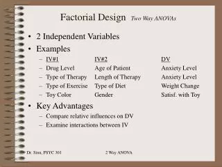
Two-Way (Independent) ANOVA. Two-Way ANOVA. “Two-Way” means groups are defined by 2 independent variables. These IVs are typically called factors . An experiment in which any combination of values for the 2 factors can occur is called a completely crossed factorial design.

Two-Way (Independent) ANOVA
E N D
Presentation Transcript
Two-Way ANOVA • “Two-Way” means groups are defined by 2 independent variables. • These IVs are typically called factors. • An experiment in which any combination of values for the 2 factors can occur is called a completely crossed factorial design. • If all cells have the same n, the design is said to be balanced. • Still have only 1 dependent variable PSYC 6130A, PROF. J. ELDER
500 ms 500 ms 200 ms Until Response Example: Visual Grating Detection in Noise PSYC 6130A, PROF. J. ELDER
2 x 3 Design 0.5 Grating Frequency (c/deg) 1.7 50.0% 4.3% 14.8% Noise Contrast PSYC 6130A, PROF. J. ELDER
Balanced Design Factor B Factor A PSYC 6130A, PROF. J. ELDER
Descriptive Statistics PSYC 6130A, PROF. J. ELDER
Interactions • If there is no interaction between the factors (spatial frequency, noise contrast), the dependent variable (SNR) for each condition (cell) can be predicted from the independent effects of factors A and B: • Cell mean = Grand mean + Row effect + Column effect PSYC 6130A, PROF. J. ELDER
Interactions • If there are no interactions, curves should be parallel (effect of noise contrast is independent of spatial frequency). PSYC 6130A, PROF. J. ELDER
Types of Effects PSYC 6130A, PROF. J. ELDER
Interactions • In the general case, Cell mean = Grand mean + Row effect + Column effect + Interaction effect • Score deviations from cell means are considered error (unpredictable). • Thus: Score = Grand mean + Row effect + Column effect + Interaction effect + Error • OR Score - Grand mean = Row effect + Column effect + Interaction effect + Error PSYC 6130A, PROF. J. ELDER
Sum of Squares Analysis PSYC 6130A, PROF. J. ELDER
Single Subscript Notation PSYC 6130A, PROF. J. ELDER
Double Subscript Notation PSYC 6130A, PROF. J. ELDER
Double Subscript Notation • The first subscript refers to the row that the particular value is in, the second subscript refers to the column. PSYC 6130A, PROF. J. ELDER
Double Subscript Notation • Test your understanding by identifying in the table below. PSYC 6130A, PROF. J. ELDER
Double Subscript Notation • We will follow the notation of Howell: PSYC 6130A, PROF. J. ELDER
Multi-Subscript Notation • In two-way ANOVA, 3 indices are needed: PSYC 6130A, PROF. J. ELDER
Multi-Subscript Notation • Statistics are calculated by summing over scores within cells, and thus the third subscript (k) is dropped: PSYC 6130A, PROF. J. ELDER
Multi-Subscript Notation PSYC 6130A, PROF. J. ELDER
Pooled Statistics • Multi-factor ANOVA requires the calculation of statistics that pool, or ‘collapse’ data over one or more factors. • We indicate the factors over which the data are being pooled by substituting a ‘bullet’ • for the corresponding index. PSYC 6130A, PROF. J. ELDER
Pooled Statistics PSYC 6130A, PROF. J. ELDER
Group Noise Contrast (Michelson units) Total .043 .148 .500 Mean Mean Mean Mean Spatial Frequency .500 Signal to Noise 7.8 6.4 6.5 6.9 (cpd) at Threshold (%) 1.700 9.5 8.9 9.8 9.4 Group Total 8.7 7.6 8.2 8.2 Noise Contrast (Michelson units) .043 .148 .500 Std Deviation Std Deviation Std Deviation Spatial .500 Signal to Noise 0.62 0.29 0.31 Frequency at Threshold (cpd) 1.700 Signal to Noise 0.36 0.54 0.80 at Threshold Example PSYC 6130A, PROF. J. ELDER
Step 1. State the Hypothesis • Null hypothesis has 3 parts, e.g., • Mean SNR at threshold same for both spatial frequencies • Mean SNR at threshold same for all noise levels • No interactions PSYC 6130A, PROF. J. ELDER
Step 2. Select Statistical Test and Significance Level • Normally use same a-level for testing all 3 F ratios. PSYC 6130A, PROF. J. ELDER
Step 3. Select Samples and Collect Data • Strive for a balanced design • Ideally, randomly sample • More probably, random assignment PSYC 6130A, PROF. J. ELDER
Generally have 3 different critical values for each F test Numerator Step 4. Find Regions of Rejection Denominator PSYC 6130A, PROF. J. ELDER
Degrees of Freedom Tree PSYC 6130A, PROF. J. ELDER
Step 5. Calculate the Test Statistics PSYC 6130A, PROF. J. ELDER
Step 5. Calculate the Test Statistics PSYC 6130A, PROF. J. ELDER
Step 6. Make the Statistical Decisions • Note that 3 independent statistical decisions are being made. • Thus the probability of one or more Type I errors is greater than the α value used for each test. • It is not common to correct for this. • You should be aware of this issue as both a producer and consumer of scientific results! PSYC 6130A, PROF. J. ELDER
Main effects Interaction SPSS Output PSYC 6130A, PROF. J. ELDER
SPSS Output PSYC 6130A, PROF. J. ELDER
Assumptions of Two-Way Independent ANOVA • Same as for One-Way • If balanced, don’t have to worry about homogeneity of variance. PSYC 6130A, PROF. J. ELDER
Advantages of 2-Way ANOVA with 2 Experimental Factors • One factor may not be of interest (e.g., gender), but may affect the dependent variable. • Explicitly partitioning the data according to this ‘nuisance’ variable can increase the power of tests on the independent variable of interest. PSYC 6130A, PROF. J. ELDER
Simple Effects • When significant main effects are discovered, it is common to also test for simple effects. PSYC 6130A, PROF. J. ELDER
Simple Effects • A main effect is an effect of one factor measured by collapsing (pooling) over all other factors. • A simple effect is an effect of one factor measured by fixing all other factors. • Although we found significant main effects, given the significant interaction, these main effects do not necessarily imply similarly significant simple effects. PSYC 6130A, PROF. J. ELDER
Simple Effects • Thus, particularly when a significant interaction is observed, a factorial ANOVA is often followed up by a series of one-way ANOVAS to test simple effects. • For our example, there are a total of 5 possible simple effects to test. PSYC 6130A, PROF. J. ELDER
Simple Effects • To conduct follow-up one-way ANOVA tests of simple effects in SPSS: • Select Split File … from the Data menu • Click on Organize Output by Groups • Transfer the factor to be held constant to the space labeled “Groups Based On.” • Now proceed with one-way ANOVAS as usual. PSYC 6130A, PROF. J. ELDER
a Test of Homogeneity of Variances Signal to Noise at Threshold a ANOVA Levene Statistic df1 df2 Sig. Signal to Noise at Threshold 5.120 2 27 .013 Sum of a. Spatial Frequency (cpd) = .500 Squares df Mean Square F Sig. Between Groups .001 2 .001 32.990 .000 Within Groups .001 27 .000 Total .002 29 a. Spatial Frequency (cpd) = .500 b Robust Tests of Equality of Means Signal to Noise at Threshold a Statistic df1 df2 Sig. Welch 21.413 2 16.975 .000 Brown-Forsythe 32.990 2 17.382 .000 a. Asymptotically F distributed. b. Spatial Frequency (cpd) = .500 Simple Effects PSYC 6130A, PROF. J. ELDER
a Test of Homogeneity of Variances Signal to Noise at Threshold Levene Statistic df1 df2 Sig. 2.037 2 27 .150 a. Spatial Frequency (cpd) = 1.700 a ANOVA Signal to Noise at Threshold Sum of Squares df Mean Square F Sig. Between Groups .000 2 .000 5.899 .007 Within Groups .001 27 .000 Total .001 29 a. Spatial Frequency (cpd) = 1.700 b Robust Tests of Equality of Means Signal to Noise at Threshold a Statistic df1 df2 Sig. Welch 5.527 2 16.511 .015 Brown-Forsythe 5.899 2 19.883 .010 a. Asymptotically F distributed. b. Spatial Frequency (cpd) = 1.700 Simple Effects PSYC 6130A, PROF. J. ELDER
Simple Effects • Again note that multiple independent statistical decisions are being made. • Conditioning the test for simple effects on a significant main effect provides protection if only 2 simple effects are being tested. • Otherwise, the probability of one or more Type I errors is greater than the α value used for each test. • It is not common to correct for this. • You should be aware of this issue as both a producer and consumer of scientific results! PSYC 6130A, PROF. J. ELDER
End of Lecture April 8, 2009
Planned or Posthoc Pairwise Comparisons • If significant main (and possibly simple) effects are found, it is common to follow up with one or more pairwise tests. • It is most common to test differences between marginal means within a factor (i.e., pooling over the other factor). • In this example, there are only 3 meaningful posthoc tests on marginal means. Why? PSYC 6130A, PROF. J. ELDER
Test of Homogeneity of Variances Signal to Noise at Threshold Levene Multiple Comparisons Statistic df1 df2 Sig. Dependent Variable: Signal to Noise at Threshold 12.229 2 57 .000 LSD Mean 95% Confidence Interval (I) Noise Contrast (J) Noise Contrast Difference (Michelson units) (Michelson units) (I-J) Std. Error Sig. Lower Bound Upper Bound .043 .148 .010120 * .004492 .028 .00112 .01912 .500 .004800 .004492 .290 -.00420 .01380 .148 .043 -.010120 * .004492 .028 -.01912 -.00112 .500 -.005320 .004492 .241 -.01432 .00368 .500 .043 -.004800 .004492 .290 -.01380 .00420 .148 .005320 .004492 .241 -.00368 .01432 *. The mean difference is significant at the .05 level. Pairwise Comparisons on Marginal Means • Since there are 3 levels of noise, we can consider using Fisher’s LSD. • However, since variances do not appear homogeneous, we should not use an LSD based on pooling the variance over all 3 conditions. PSYC 6130A, PROF. J. ELDER
Multiple Comparisons Dependent Variable: Signal to Noise at Threshold Games-Howell Mean 95% Confidence Interval (I) Noise Contrast (J) Noise Contrast Difference (Michelson units) (Michelson units) (I-J) Std. Error Sig. Lower Bound Upper Bound .043 .148 .010120 * .003787 .030 .00085 .01939 .500 .004800 .004573 .552 -.00648 .01608 .148 .043 -.010120 * .003787 .030 -.01939 -.00085 .500 -.005320 .005028 .546 -.01762 .00698 .500 .043 -.004800 .004573 .552 -.01608 .00648 .148 .005320 .005028 .546 -.00698 .01762 *. The mean difference is significant at the .05 level. Pairwise Comparisons on Marginal Means • Alternative when variances appear heterogeneous: • Compute Fisher’s LSD by hand, calculating standard error separately for each test (not difficult) • One of the unequal variance post-hoc tests offered by SPSS PSYC 6130A, PROF. J. ELDER
Planned or Posthoc Pairwise Comparisons • It is also possible to test differences between cell means. Note that in this design, there are 15 possible pairwise cell comparisons. • It doesn’t make that much sense to compare 2 cells that are not in the same row or column (i.e. that differ in both factors). • It is more likely that you would follow a significant simple effect test with a set of pairwise comparisons within a factor while holding the other factor constant. There are 9 such comparisons possible here. • For example, within a spatial frequency condition, what noise conditions differ significantly? • This defines a total of 6 pairwise comparisons (2 families of 3 comparisons each). PSYC 6130A, PROF. J. ELDER
a Multiple Comparisons Dependent Variable: Signal to Noise at Threshold Games-Howell Mean 95% Confidence Interval (I) Noise Contrast (J) Noise Contrast Difference (Michelson units) (Michelson units) (I-J) Std. Error Sig. Lower Bound Upper Bound .043 .148 .005890 * .002067 .030 .00055 .01123 .500 -.003160 .002790 .513 -.01056 .00424 .148 .043 -.005890 * .002067 .030 -.01123 -.00055 .500 -.009050 * .003066 .024 -.01697 -.00113 .500 .043 .003160 .002790 .513 -.00424 .01056 .148 .009050 * .003066 .024 .00113 .01697 *. The mean difference is significant at the .05 level. a. Spatial Frequency (cpd) = 1.700 Planned or Posthoc Pairwise Comparisons • Alternative when variances appear heterogeneous: • Compute Fisher’s LSD by hand, calculating standard error separately for each test (not difficult) • One of the unequal variance post-hoc tests offered by SPSS (assumes all-pairs) PSYC 6130A, PROF. J. ELDER
Interaction Comparisons • If significant interactions are found in a design that is 2x3 or larger, it may be of interest to test the significance of smaller (e.g., 2x2) interactions. • These can be tested by ignoring specific subsets of the data for each test (e.g., by using the SPSS Select Cases function). PSYC 6130A, PROF. J. ELDER