Download
1 / 10
110 likes | 231 Vues
This resource provides an introduction to statistical methods for analyzing count data using R, tailored for students and researchers at the University of Sunderland. It covers special types of data, including counts, proportions, survival analysis, and binary responses. Key topics include handling count data with generalized linear models (GLMs) using the Poisson and quasipoisson families, as well as contingency tables and ANCOVA techniques. Practical examples highlight the use of R functions such as `table()`, `tapply()`, and plotting methods for meaningful insights.

E N D
Count Data Harry R. Erwin, PhD School of Computing and Technology University of Sunderland
Resources • Crawley, MJ (2005) Statistics: An Introduction Using R. Wiley. • Freund, RJ, and WJ Wilson (1998) Regression Analysis, Academic Press. • Gentle, JE (2002) Elements of Computational Statistics. Springer. • Gonick, L., and Woollcott Smith (1993) A Cartoon Guide to Statistics. HarperResource (for fun).
Introduction • These four demonstration sessions of this class address special types of data: • Counts • Proportions • Survival analysis • Binary responses
Frequencies and Proportions • With frequency data, we know how often something happened, but not how often it didn’t happen. • With proportion data (next week), we know how often it didn’t happen.
Count Data • Linear regression assumes constant variance and normal errors. This is not appropriate for count data: • Counts are non-negative. • Response variance usually increases with the mean. • Errors are not normally distributed. • Zeros are hard to transform.
Handling Count Data in R • Use a glmwith family=poisson. • This sets errors to Poisson, so variance is proportional to the mean. • This sets link to log, so fitted values are positive. • Book example • If you have overdispersion (residual deviance greater than residual degrees of freedom), use family=quasipoisson.
Analysis of Count Data • Book example (230ff) • Use of table() • Use of tapply() • fitting the glm with family = poisson. • refitting with family = quasipoisson. • three and four-way interactions • model simplification • documentation
Contingency Tables • Risk of data aggregation over important explanatory variables (nuisance variables) • Book example (234ff) • The saturated model • Remove the N-way interaction and see if it was significant. • If the N-way interaction is significant, go no further. • Then remove the scientifically interesting interaction and see if it is significant. • You have to check the nuisance variables first!
ANCOVA with Counts • Book example (237ff) • plotting and use of split to gain insight. • analysis—testing for the need for different slopes. • use of predict() to draw lines through the plot.
Frequency Distributions • Book example (240ff) • testing for independence • use of table() • use of dpois() • plotting and interpretation • use the negative binomial distribution for data with variance much greater than the mean • use the binomial distribution for data with variance less than the mean