Download
1 / 54
580 likes | 977 Vues
A Brief of Molecular Evolution & Phylogenetics. Aims of the course:. To introduce to the practice phylogenetic inference from molecular data. To known applications and computer programmes to practice phylogenetic inference. Two Concepts of Molecular Evolution. Ortologous vs Paralogous genes

E N D
Aims of the course: • To introduce to the practice phylogenetic inference from molecular data. • To known applications and computer programmes to practice phylogenetic inference.
Two Concepts of Molecular Evolution • Ortologous vs Paralogous genes • Genes & species trees • Molecular clock • Substitution rates
Homologous genes • Orthologous genes Derived from a process of new species formation (speciation) • Paralogous genes Derived from an original gene duplication process in a single biological species
Species trees vs Gene trees • Paralogous genes of Globin • a, b, d (Glob), Myo y Leg haemoglobin, each originated by duplication from an ancestral gene Orthologous genes of Cytochrome Each one is present in a biological species
Species trees and Gene trees A a Species tree Gene tree B b D c We often assume that gene trees give us species trees
Orthologues and paralogues paralogous b* C* A* orthologous orthologous c C* B A* a b* A mixture of orthologues and paralogues sampled Duplication to give 2 copies = paralogues on the same genome Ancestral gene
The malic enzyme gene tree contains a mixture of orthologues and paralogues Gene duplication Anas = a duck! Plant chloroplast Plant mitochondrion
Is there a molecular clock? • The idea of a molecular clock was initially suggested by Zuckerkandl and Pauling in 1962 • They noted that rates of amino acid replacements in animal haemoglobins were roughly proportional to time - as judged against the fossil record
The molecular clock for alpha-globin:Each point represents the number of substitutions separating each animal from humans shark carp number of substitutions platypus chicken cow Time to common ancestor (millions of years)
Rates of amino acid replacement in different proteins • Evolutionary rates depends on functional constraints of proteins
There is no universal clock • The initial proposal saw the clock as a Poisson process with a constant rate • Now known to be more complex - differences in rates occur for: • different sites in a molecule • different genes • different base position (synonimous-nonsynonymous) • different regions of genomes • different genomes in the same cell • different taxonomic groups for the same gene • Molecular Clocks Not Exactly Swiss
Phylogenetic Trees LEAVES terminal branches A B C D E F G H I J node 2 node 1 polytomy interior branches A CLADOGRAM ROOT
Trees - Rooted and Unrooted A B C D E F G H I J B C D E I G A H J F ROOT ROOT E D ROOT F A H J B G C I
eukaryote eukaryote eukaryote eukaryote Rooting using an outgroup archaea archaea Unrooted tree archaea Rooted by outgroup bacteria Outgroup archaea Monophyletic Ingroup archaea archaea eukaryote Monophyletic Ingroup eukaryote root eukaryote eukaryote
Distance Methods • Distance Estimates attempt to estimate the mean number of changes per site since 2 species (sequences) split from each other. • Simply counting the number of differences may underestimate the amount of change - especially if the sequences are very dissimilar - because of multiple hits. • We therefore use a model which includes parameters which reflect how we think sequences may have evolved.
Cálculo de distancias: observación y realidad 1 2 obs real sustitución: A A A A 0 0no A A A C 1 1simple A C A G 1 2coincidente A A A C G 1 2múltiple A C A C 0 2paralela A C A G C 0 3convergente A A A C A 0 2reversa
The simplest model : Jukes & Cantor:dxy = -(3/4) Ln (1-4/3 D) • dxy= distance between sequence x and sequence y expressed as the number of changes per site • (note dxy= r/n where r is number of replacements and n is the total number of sites. This assumes all sites can vary and when unvaried sites are present in two sequences it will underestimate the amount of change which has occurred at variable sites) • D = is the observed proportion of nucleotides which differ between two sequences (fractional dissimilarity) • Ln = natural log function to correct for superimposed substitutions • The 3/4 and 4/3 terms reflect that there are four types of nucleotides and three ways in which a second nucleotide may not match a first - with all types of change being equally likely (i.e. unrelated sequences should be 25% identical by chance alone)
The natural logarithm ln is used to correct for superimposed changes at the same site • If two sequences are 95% identical they are different at 5% or 0.05 (D) of sites thus: • dxy = -3/4 ln (1-4/3 0.05) = 0.0517 • Note that the observed dissimilarity 0.05 increases only slightly to an estimated 0.0517 - this makes sense because in two very similar sequences one would expect very few changes to have been superimposed at the same site in the short time since the sequences diverged apart • However, if two sequences are only 50% identical they are different at 50% or 0.50 (D) of sites thus: • dxy = -3/4 ln (1-4/3 0.5) = 0.824 • For dissimilar sequences, which may diverged apart a long time ago, the use of ln infers that a much larger number of superimposed changes have occurred at the same site
Distance models can be made more parameter rich to increase their realism 1 • It is better to use a model which fits the data than to blindly impose a model on data • The most common additional parameters are: • A correction for the proportion of sites which are unable to change • A correction for variable site rates at those sites which can change • A correction to allow different substitution rates for each type of nucleotide change • PAUP will estimate the values of these additional parameters for you.
A gamma distribution can be used to model site rate heterogeneity
Exchangeability parameters for two models of amino acidreplacement. Exchangeability parameters from two common empiricalmodels of amino acid sequence evolution are presented. Theparameter value for each amino acid pair is indicated by the areas ofthe bubbles, and discounts the effects of amino acid frequencies. (a) The JTT model (Jones, D.T. et al. 1992CABIOS 8, 275–282) derived from a wide variety of globular proteins. (b) The mtREV model (Yang, Z. et al. 1998 Mol. Biol. Evol.15, 1600–161) derived from mammalian mitochondrial genesthat encode various transmembrane proteins.
Distances: advantages: • Fast - suitable for analysing data sets which are too large for ML • A large number of models are available with many parameters - improves estimation of distances • Use ML to test the fit of model to data
Distances: disadvantages: • Information is lost - given only the distances it is impossible to derive the original sequences • Only through character based analyses can the history of sites be investigated e,g, most informative positions be inferred. • Generally outperformed by Maximum likelihood methods in choosing the correct tree in computer simulations
Numbers of possible trees for N taxa: • T(i) = P (2i-5) :: T(unrooted), i>3 1,3,15,105,945,10395,135135 • For 10 taxa there are 2 x 10⁶ unrooted trees • For 50 taxa there are 3 x 1074 unrooted trees • How can we find the best tree ?
Cluster Analysis UPGMA y NJ Se unen recursivamente el par de elementos más cercanos. Se recalcula la matriz de distancias (*) y seanaliza el par unido como un nuevo elemento
Unrooted Neighbor-Joining Tree Human Spinach Monkey Mosquito Rice
C A 0.1 0.2 0.3 0.1 0.6 D B A perfectly additive tree A B C D A - 0.4 0.4 0.8 B 0.4 - 0.6 1.0 C 0.4 0.6 - 0.8 D 0.8 1.0 0.8 - The branch lengths in the matrix and the tree path lengths match perfectly - there is a single unique additive tree
Distance estimates may not make an additive tree Aquifex > Bacillus (0.335) Some path lengths are longer and others shorter than appear in the matrix Aquifex > Thermus (0.33) Jukes-Cantor distance matrix Proportion of sites assumed to be invariable = 0.56; identical sites removed proportionally to base frequencies estimated from constant sites only 1 2 4 5 6 1 ruber - 2 Aquifex 0.38745 - 4 Deinococc 0.22455 0.47540 - 5 Thermus 0.13415 0.273130.23615 - 6 Bacillus 0.27111 0.33595 0.28017 0.28846 - Thermus > Deinococcus (0.218)
Obtaining a tree using pairwise distances • Stochastic errors will cause deviation of the estimated distances from perfect tree additivity even when evolution proceeds exactly according to the distance model used • Poor estimates obtained using an inappropriate model will compound the problem • How can we identify the tree which best fits the experimental data from the many possible trees
Obtaining a tree using pairwise distances • Use statistics to evaluate the fit of tree to the data (goodness of fit measures) • Fitch Margoliash method - a least squares method • Minimum evolution method - minimises length of tree • Note that neighbor joining while fast does not evaluate the fit of the data to the tree
Fitch Margoliash Method 1968: • Minimises the weighted squared deviation of the tree path length distances from the distance estimates
Fitch Margoliash Method 1968: Tree 2 - best Tree 1 Optimality criterion = distance (weighted least squares with power=2) Score of best tree(s) found = 0.12243 (average %SD = 11.663) Tree # 1 2 Wtd. S.S. 0.13817 0.12243 APSD 12.391 11.663
Minimum Evolution Method: • For each possible alternative tree one can estimate the length of each branch from the estimated pairwise distances between taxa and then compute the sum (S) of all branch length estimates. The minimum evolution criterion is to choose the tree with the smallest S value
Minimum Evolution Tree 2 Tree 1 - best Optimality criterion = distance (minimum evolution) Score of best tree(s) found = 0.68998 Tree # 1 2 ME-score 0.68998 0.69163
Parsimony analysis • Parsimony methods provide one way of choosing among alternative phylogenetic hypotheses • The parsimony criterion favours hypotheses that maximise congruence and minimise homoplasy (convergence, reversal & parallelism) • It depends on the idea of the fit of a character to a tree
C A T A C T 3(A) 1(C) 1(C) 3(A) A A 4(C) 2(A) 4(C) 2(A) 2 mutations 1 mutation Parsimony Seq 1 ...ACCT... Seq 2 ...AACT... Seq 3 ...TACT... Seq 4 ...TCCT... 1 2 0 0 = 3
Maximum Likelihood - goal • To estimate the probability that we would observe a particular dataset, given a phylogenetic tree and some notion of how the evolutionary process worked over time. • P(D/H) given Probability of
Maximum likelihood Where: gx0prior probability that node 0 has nucleotide x (relative frequency) 3 1 5 6 V1 V3 V5 V4 V2 (if gi=1/4, model becomes JC) 4 2 Since we do not know x5 and x6 we sum over all the possible nucleotides Summing over all sites: lnL is maximized changing Vi’s
Bayes’ theorem Posterior distribution Prior distribution Likelihood function Unconditional probab. Pr [Tree/Data] = (Pr [Tree] x Pr [Data/Tree]) / Pr [Data])
B C A 1.0 probability Prior probability distribution Data (observations) 1.0 probability Posterior probability distribution
Markov Chain Monte Carlo (MCMC) probability parameter space
Bootstrap ...ahhfhgkhkafdggg... ...rhhfkgkhkaydggg... ...ahhfhgk-kafdggg... ...ahhfhgk-kafdggg... ...ghhfhg--kafdhtt... ...ahhfhg--kafddgg... ...hhhfhg--kafddgg... ...ahhfpgchka-wggg... ...ahdfhgkhkafkdgg... ...rhdfkgkhkaykdgg... ...ahdfhgk-kafkdgg... ...ahdfhgk-kafkdgg... ...ghdfhg--kafkdht... ...ahdfhg--kafaddg... ...hhdfhg--kafaddg... ...ahdfpgchka-kwgg... 86 50 75 90 .... 70 65 ...adfhgkkaffkdgg... ...rdfkgkkayykdgg... ...adfhgkkaffkdgg... ...adfhgkkaffkdgg... ...gdfhg-kaffkdht... ...adfhg-kaffaddg... ...hdfhg-kaffaddg... ...adfpgcka--kwgg...
Aplicaciones de la filogenia: Trazar el origen de una cepa Fechar la introducción de una cepa Estudio de la función Estudios evolutivos
Trazando el origen Europa Asia América Europa
Datos epidemiológicos Virus RNA: alta tasa de evolución t1 b c 1970 (1926-t0)*v=a (1970-t1)*v=c+d ... d a 1926 t0