Download
1 / 47
500 likes | 829 Vues
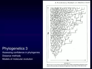
Phylogenetics 3 Assessing confidence in phylogenies Distance methods Models of molecular evolution . Estimating confidence in tree topologies Congruence Consensus trees The bootstrap applied to phylogenetics Bremer support (the Decay Index)

E N D
Phylogenetics 3 Assessing confidence in phylogenies Distance methods Models of molecular evolution
Estimating confidence in tree topologies Congruence Consensus trees The bootstrap applied to phylogenetics Bremer support (the Decay Index) Distance methods and models of molecular evolution General introduction to distance methods Distance transformations and introduction to models of molecular evolution Phylogenetic clustering methods using distances
Just because you have the shortest tree, how do you know it is correct? Of course, you will never know with absolute certainty that it is correct, but there are various methods for assessing confidence… Ways of measuring support • Congruence among independent datasets (but not multiple analyses of the same data) • e.g., multiple independent loci, molecular and morphological data • Bootstrap support • nonparametric way to assess relative branch support applicable to all optimality criteria (jacknife support is similar) • Bremer support • parsimony-based measure of relative branch support • Posterior probabilities • will discuss later © Paul Lewis
Consensus trees are used to display congruence among trees graphically Consensus trees summarize information in multiple trees (e.g., multiple equally parsimonious trees, bootstrap trees, etc). Strict and Majority Rule are the most commonly employed consensus methods, but there are others. Li and Graur Fig. 5.25
Bootstrapping is a statistical resampling technique used to assess confidence. Bootstrapping Suppose you sequence the 18S rRNA gene and estimate the tree. What tree would you have estimated had you chosen a different gene to sequence? Which parts of the tree (i.e. splits) would you expect to be present in trees estimated from genes like the one you sampled? Felsenstein, J. 1985. Confidence intervals on phylogenies: an approach using the bootstrap. Evolution 39:783-791. © Paul Lewis
It is not possible to rerun evolution and generate independent replicates of the data. So, bootstrapping uses “pseudosamples” to obtain the variance of the estimate of the phylogeny. Swofford et al. Fig. 33
Another representation of the bootstrap Li and Graur Fig. 5.26
1 2 3 4 Bootstrapping can also be thought of as an exercise in reweighting of characters... Bootstrapping: first step There are k characters in this dataset, each with a weight of 1 From the original data, estimate a tree using, say, parsimony (could use NJ, LS, ML, etc., however) © Paul Lewis
1 2 3 4 Bootstrapping: first replicate Sum of weights equals k (i.e., each bootstrap dataset has same number of sites as the original) From the bootstrap dataset, estimate the tree using the same method you used for the original dataset © Paul Lewis
1 3 2 4 Bootstrapping: second replicate Note that weights are different this time, reflecting the random sampling with replacement used to generate the weights This time the tree that is estimated is different than the one estimated using the original dataset. © Paul Lewis
1 1 1 2 2 2 4 4 4 3 3 3 1 1 1 1 1 1 1 1 1 1 1 1 1 1 1 1 2 2 2 3 2 2 2 2 2 2 2 2 2 2 2 2 1 3 3 2 3 3 3 3 3 3 3 3 3 3 3 3 3 3 4 4 4 4 4 4 4 4 4 4 4 4 4 4 4 4 2 4 Bootstrapping: 20 replicates • Freq • ---------- • -*-* 75.0 • -**- 15.0 • --** 10.0 Note: usually at least 100 replicates are performed, and 500 is better © Paul Lewis
Bootstrap results are usually visualized as majority-rule consensus trees. Bootstrap values may be displayed on the MR consensus, or may be indicated on the optimal tree. Left: Phylogram (tree with branch lengths drawn proportional to amounts of change/genetic distance) with bootstrap values placed along branches. Right: Corresponding 50% majority-rule consensus tree, with branches supported by <50% of the bootstrap replicates collapsed. Li and Graur Fig. 5.27
Bootstrapping Comments • This type of bootstrapping is nonparametric (no assumptions have been made about the probability distribution underlying the data) • Assumes the sites you have sampled are representative • Bootstrap values are not equivalent to p values or probabilities • High bootstrap values are probably too high, and low bootstraps are too low (based on simulation experiments) • 80-85% seems to be generally accepted as a good minimum trustworthy bootstrap value • Bootstrapping is a lot of work (must perform at least 100 searches) © Paul Lewis
Nodal support? 1 2 3 4 “This node (ancestor to 3 and 4) has 95% bootstrap support” 95 The above statement makes sense only if rooting is correct... © Paul Lewis
...or branch support? 4 3 1 2 Now it is the ancestor of 1 and 2 that that has 95% bootstrap support 95 Saying that the branch (or split) has 95% bootstrap support always works © Paul Lewis
Bremer Support (aka the Decay Index) An alternative measure of confidence (robustness) based on parsimony. The universe of trees from analysis of a dataset on algae 2 most-parsimonious trees No. trees 411 414 415 416 417 418 next-best tree 3 steps longer Tree length © Paul Lewis
411 steps 415 steps Strict consensus made from sets of trees up to 425 steps 424 steps 425 steps 416 steps Consensus trees become progressively less resolved as the allowable length of the input trees increases. © Paul Lewis
The Bremer support value for a branch is the number of extra steps needed before finding trees that lack that branch 14 13 4 5 © Paul Lewis
Here bootstrap values (%) are shown for comparison 14 100% 100% 13 5 4 74% 76% © Paul Lewis
Estimating confidence in tree topologies Congruence Consensus trees The bootstrap applied to phylogenetics Bremer support (the Decay Index) Distance methods and models of molecular evolution General introduction to distance methods Distance transformations and introduction to models of molecular evolution Phylogenetic clustering methods using distances
Distance methods • 1. General introduction • Distance methods for phylogenetic reconstruction involve analyses of pairwise distance matrices—each cell is a distance between one pair of taxa. • Some kinds of phylogenetic data are inherently composed of pairwise distances, such as DNA-DNA hybridization data (no longer widely used). Discrete character data, such as DNA or amino acid sequences, must be transformed into distances. • Distance transformations for molecular data are often based on models of molecular evolution (more on models later) • Thus, a distance analysis of molecular sequences involves three steps: • Sequence alignment • Distance transformation • Estimation of trees (may involve sequential recalculation of distances) • Whereas, a discrete character-based method involves two steps • Sequence alignment • Estimation of trees Swofford et al. p. 487
1 3 a d c b e 4 2 Phylogenetic analyses using distance methods convert distance measures in a distance matrix (dij) into path lengths on a phylogenetic tree (pij). p12 = a + b p23 = b + c + d Perfect distance data have perfect additivity, meaning that for every pair of taxa, dij = pij Real data never have perfect additivity. Some clustering methods involve optimality criteria that measure the departure from additivity p13 = a + c + d p24 = b + c + e p14 = a + c + e p34 = d + e © Paul Lewis
Advantages of distance methods • Fast (significant, especially when using bootstrapping) • Allow use of models of molecular evolution • Disadvantages of distance methods • Distances may not capture all the information about sequence variation • Tree inference is decoupled from inferences about evolution of individual characters (e.g., no way to determine which sites are evolving at high/low rates) • Hard to combine different types of data (e.g., molecules/morphology; nucleotides/amino acids)
2. Distance transformations for molecular data, and introduction to models of molecular evolution A divergence matrix provides a general framework for describing distance transformations for sequence data. Consider two sequences with an aligned length of N positions. Each cell in the divergence matrix is the frequency with which a pair of nucleotides occurs at each aligned positions Swofford et al. p. 454
The simplest distance transformation: • Uncorrected distance, aka dissimilarity or “p-distance” • = Total number of differences divided by total number of sites • Referring back to the divergence matrix, the p-distance is: • If the sequences are identical, the a, f, k, p values will sum to 1, and the p-distance will be zero. • If the sequences have no positions with the same nucleotides, the off-diagonal values will sum to 1, and the p-distance will be one (can this result ever be obtained?). Swofford et al. p. 454-5
A A A Problems with p-distances: Multiple hits destroy additivity Over short evolutionary timescales, the number of differences observed in two aligned sequences will be approximately equal to the number of substitutions that actually occurred along the branches of the tree separating those sequences. But, over long evolutionary timescales, there may be multiple substitutions (“multiple hits”) at the same sites, which will cause the observed differences to underestimate the actual number of substitutions that have occurred G G G A A → G A → G Similarity expected for short divergences A → G Unfortunately, some similarity is also expected for long divergences. Molecular homoplasy! Impossible to detect a priori, because characters are so simple (ACGT) Difference expected for long divergences © Paul Lewis A A
Additivity: time ≈ substitutions additivity nonadditivity substitutions time increasing, but number of observed substitutions staying constant number of observed substitutions is more or less linear wrt time Time since common ancestor © Paul Lewis
Over a really, really long time... A A If a really large number of substitutions have occurred, it no longer matters what base we started with Probability of seeing same state at both ends is thus 1/4 (if base frequencies are equal) Probability of seeing a difference is thus 3/4 Bottom line: 1/4 of the similarities are misleading because they are due to chance © Paul Lewis
Another way to say the same thing as the previous slide… Probability of “A present” as a function of time Upper curve assumes we started with A at time 0. Over time, the probability of still seeing an A at this site drops because rate of changing to one of the other three bases is 3a (so rate of staying the same is -3a). The equilibrium relative frequency of A is 0.25 Lower curve assumes we started with some state other than A (T is used here). Over time, the probability of seeing an A at this site grows because the rate at which the current base will change into an A is a. © Paul Lewis
Distance transformations that “correct” for multiple hits based on models of molecular evolution can make p-distances more additive. Jukes-Cantor (JC69) one-parameter model Assumes that all transformations between nucleotides occur at the same rate Kimura (K80 or K2P) two-parameter model Assumes that transitions and transversions occur at different rates AC AC Transitions Transversions GT GT K2P JC69
Models of molecular evolution are based on matrices that specify transformation rates. Models vary in the numbers and kinds of parameters used to determine elements in the rate matrix JC69* rate matrix 1 parameter: a “To” state “From” state *Jukes, T. H., and C. R. Cantor. 1969. Evolution of protein molecules. Pages 21-132 in H. N. Munro (ed.), Mammalian Protein Metabolism. Academic Press, New York. © Paul Lewis
nonadditivity additivity substitutions time Models increase additivity by increasing larger p-distances more than smaller ones d = -¾ln(1 - 4p/3) Jukes-Cantor distance vs p-distance © Paul Lewis
K80* (or K2P) rate matrix 2 parameters: a b “To” state rate of transversions is b rate of transitions is a “From” state The diagonal elements make rows sum to 0 *Kimura, M. 1980. A simple method for estimating evolutionary rate of base substitutions through comparative studies of nucleotide sequences. Journal of Molecular Evolution 16:111-120. © Paul Lewis
K80 rate matrix (looks different, but really the same) 2 parameters: k b rate of transversions is b rate of transitions is kb All I’ve done is re-parameterize the rate matrix, letting k equal the transition/transversion rate ratio Note: the K80 model is identical to the JC69 model if k = 1 (a = b) © Paul Lewis
Distance correction for K80 (K2P) model: This distance correction separates the proportion of transitions (P) vs. transversions (Q) and reflects the principle that these types of substitutions occur at different rates. Distances estimated with the K80 (two parameter) correction may differ from those estimated with JC69 (one parameter) correction, especially when sequences are long, and divergences are great. Swofford et al. p. 454-6
Many other models of molecular evolution have been described, not all of which have straightforward distance corrections. Examples: Felsenstein 1981 (F81) model: Transformation rates determined by mean substitution rate (m) and equilibrium base frequencies (e.g., pA) 4 parameters: pA pC pG m Identical to the JC69 model if all the base frequencies are set to ¼. *Felsenstein, J. 1981. Evolutionary trees from DNA sequences: a maximum likelihood approach. Journal of Molecular Evolution 17:368-376. © Paul Lewis
Hasegawa-Kishino-Yano 1985 (HKY85) model: Transformation rates determined by mean substitution rate (b), transition-transversion rate ratio (k) and equilibrium base frequencies (e.g., pA) 5 parameters: pA pC pG k b Identical to the F81 model if k = 1. Identical to the JC69 model if k = 1 and all the base frequencies are set to ¼. *Hasegawa, M., H. Kishino, and T. Yano. 1985. Dating of the human-ape splitting by a molecular clock of mitochondrial DNA. Journal of Molecular Evolution 21:160-174. © Paul Lewis
Generalized time reversible (GTR) model: Transformation rates determined by mean substitution rate (m), relative rate parameters (a-e) and base frequencies (e.g., pA) 9 parameters: pA pC pG a b c d e m -m (pAc + pCe + pGf) Identical to the JC69 model if a = b = c = d = e = f = 1 and all the base frequencies are set to ¼. *Lanave, C., G. Preparata, C. Saccone, and G. Serio. 1984. A new method for calculating evolutionary substitution rates. Journal of Molecular Evolution 20:86-93. © Paul Lewis
The models discussed so far, and others, are interconvertible by adding or restricting parameters.(Methods for choosing among models in phylogenetics will be discussed later.) Swofford et al. p. 434
3. Phylogenetic analyses using distance matrices UPGMA Neighbor-Joining Least-squares methods
UPGMA Unweighted pair group method using averages A purely algorithmic method that assumes constant rates of molecular evolution Given a distance matrix…Cluster the two most similar OTUs, A and B, which are now considered a single, composite taxon (AB) Recalculate distances of all OTUs, with distances to the new composite taxon (AB) calculated as the average of the distances to A and B in the prior distance matrix Continue until all taxa have been clustered. Last clustering places the root halfway between the two most dissimilar taxa (clusters) UPGMA produces midpoint-rooted trees (typically referred to as “dendrograms”; these are ultrametric trees) and has an implicit assumption that rates of evolution are constant across the phylogeny, i.e., there is a molecular clock. Swofford et al. p. 451, 487
Neighbor-Joining (NJ) A very fast (and popular) method of “star decomposition” Given a distance matrix and a completely unresolved star topology… “Decompose” the tree by sequentially clustering pairs of taxa to create internal branches At each step, cluster the pair of taxa (neighbors) that minimizes the tree length, calculated as: N = no. OTUs, dij = distance between OTUS i, j NJ produces unrooted trees in which branch lengths leading to sister taxa may be unequal (i.e., there is no assumption of a molecular clock). Although NJ uses the sum of branch lengths as a criterion for selecting each pair of “neighbors” it is nonetheless an algorithmic method that does not employ an optimality criterion for choosing among trees. A pair of neighbors that is clustered during NJ analysis cannot be “unclustered”. Li and Graur p. 188, 189.
1 3 a d c b e 4 2 Fitch-Margoliash and related methods These methods seek trees that minimize the difference between path lengths on phylogenetic trees and distances in distance matrices, using sums of squares of differences. Thus, these are distance methods that employ optimality criteria. p12 = a + b p23 = b + c + d Least squares estimates are those values of a, b, c, d and e that make the dij values closest in absolute value to the corresponding pij value. Sums of squares can be used to measure this. p13 = a + c + d p24 = b + c + e p14 = a + c + e p34 = d + e © Paul Lewis
Sum of squares The powerk is most commonly one of these choices: k = 0 Cavalli-Sforza & Edwards (1967) k = 2 Fitch & Margoliash (1967) *Cavalli-Sforza, L. L., and A. W. F. Edwards. 1967. Evolution 32:550-570. **Fitch, W. M., and E. Margoliash. 1967. Science 155:279-284. JC69 distances from primate mtDNA Data from: Brown, W., E. Prager, A. Wang, and A. Wilson. 1982. Mitochondrial DNA sequences of primates, tempo and mode of evolution. Journal of Molecular Evolution 18:225-239. © Paul Lewis
Example of poor fit (k = 0) Go 0.1 0.1 0.1 Or Hu 0.1 0.1 0.1 0.1 Ch Gi Specifying an arbitrary value (such as 0.1) for all edge lengths will very rarely provide a good fit of tree paths to distances! remember this value (at least until next slide) © Paul Lewis
Go 0.05790 0.00761 0.03691 0. 04092 0.09482 Or Hu 0.05175 0.11984 Ch Gi Least squares edge lengths (k = 0) much better! © Paul Lewis
Sources: Paul Lewis, Dept. of Ecology and Evolutionary Biology, University of Connecticut. EEB 349: Phylogenetics http://www.eeb.uconn.edu/people/plewis/index.php DL Swofford, GJ Olsen, PJ Waddell, DM Hillis. 1996. Phylogenetic Inference. Pp. 407-514 in DM Hillis, C Moritz, BK mable (eds.). Molecular Systematics 2nd Ed. Sinauer Assoc. D Graur, WH Li. 2000. Fundamentals of Molecular Evolution 2nd Ed. Sinauer Assoc. S Freeman, JC Herron. 2001. Evolutionary Analysis 2nd Ed. Prentice Hall. NA Campbell, JB Reece. 2005. Biology 7th Ed. Pearson.