Basic Detection Techniques
Basic Detection Techniques. 1b (2011/09/22): Single dish systems Theory: basic properties, sky noise, system noise, Aeff/Tsys, receiver systems, mixing, filtering, A/D conversion Case study: LOFAR Low Band Antenna. Basic Detection Techniques. Visit to Dwingeloo for APERTIF measurements

Basic Detection Techniques
E N D
Presentation Transcript
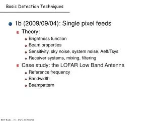
Basic Detection Techniques • 1b (2011/09/22): Single dish systems • Theory: basic properties, sky noise, system noise, Aeff/Tsys, receiver systems, mixing, filtering, A/D conversion • Case study: LOFAR Low Band Antenna
Basic Detection Techniques • Visit to Dwingeloo for APERTIF measurements • 2011/09/29 13:00-15:00 • NS to Beilen: 13:31-13:58 • NS fm Beilen: 16:59-17:28 • Transport Beilen – Dwl vv will be arranged by ASTRON • Call 0521 595119 (Diana van Dijk) in case of problems • Host is Laurens Bakker • APERTIF System Engineer)
Sensitivity • Key question: • What’s the weakest source we can observe • Key issues: • Define brightness of the source • Define measurement process • Define limiting factors in that process
Brightness function • Surface brightness: • Power received /area /solid angle /bandwidth • Unit: W m-2 Hz-1 rad-2 • Received power: • Power per unit bandwidth: • Power spectrum: w(v) • Total power: • Integral over visible sky and band • Visible sky: limited by aperture • Band: limited by receiver
Point sources, extended sources • Point source: size < resolution of telescope • Extended source: size > resolution of telescope • Continuous emission: size > field of view • Flux density: • Unit: 1 Jansky (Jy) = 10-26 W m-2 Hz-1
Reception pattern of an antenna • Beam solid angle (A = A/A0) • Measure of Field of View • Antenna theory: A0 Ωa = λ2
Black-body radiation • General: Planck’s radiation law • Radio frequencies (hv << kT): • Rayleigh-Jeans law (or rather: R-J approximation)
Antenna temperature, system temperature • Express noise power received by antenna in terms of temperature of resistor needed to make it generate the same noise power. • Spectral power: w = kT/λ2 AeffΩa = kT • Observed power: W = kT Δv • Observed flux density: S = 2kT / Aeff • Tsys = Tsky + Trec • Tsky and Tant: what’s in a name • After integration:
Sensitivity • Source power from Ta: • Source power from flux: • Antenna area A, efficiency ha • Rx accepts 1/2 radiation from unpolarized source • Define scaling factor K • K is antenna’s gain or “sensitivity” • unit: degree Jy-1
System Equivalent Flux Density • K is only related to Tant, not to Tsys • Define SEFD: • What’s in Tsys? • 3K background and Galactic radio emission Tbg • Atmospheric emission Tsky • Spill-over from the ground and other directions Tspill • Losses in feed and input waveguide Tloss • Receiver electronics Trx • At times: calibration source Tcal
High time resolution data (LOFAR // Nancay Decametric Array) Blow-up: 0.2 seconds showing complex structure