Basic Detection Techniques
Basic Detection Techniques. Detector. More than ‘sensing device’ Measuring ‘Meten is weten’ Meta information Counting vs analog. Poisson. Gaussian. Accuracy. Distribution: stochastic measurement process only ==Precision Accuracy -> no systematic Hubble Target shooting. Statistics.

Basic Detection Techniques
E N D
Presentation Transcript
Basic Detection Techniques BDT-I
Detector • More than ‘sensing device’ • Measuring • ‘Meten is weten’ • Meta information • Counting vs analog BDT-I
Poisson BDT-I
Gaussian BDT-I
Accuracy • Distribution: stochastic measurement process only • ==Precision • Accuracy -> no systematic • Hubble • Target shooting BDT-I
Statistics • Mean • Variance • Chi-squared • Median BDT-I
Moments Central moments • skewness BDT-I
Systematic errors • Instrument environment widest sense • Coal • Parallax • Gaia • Gal rotation • Pressure • Model -> none • Outliers BDT-I
Modelling • Solve • L2 (least-squares) • L1 (outliers) BDT-I
(In)direct • Direct • Raindrops • Planet directly • Indirect • Crop size • ‘systematic’ movement of Centre of G. • ‘Test particle’ BDT-I
Measurables • EM waves • Neutrinos • Matter (nuclei -> meteorites & space craft) • Gravitational waves (<=c) BDT-I
Neutrinos Weak interaction: electron neutrinos Strong interaction Tau & muon neutrinos BDT-I
Neutrinos 2 • Long pathlength -> memory • 1931: Pauli – 1959: e – 1962: new muon • Indirect • Icecube • Ocean • Moon BDT-I
Neutrino 3 • Solar problem • 1987 SN -> 19 neutrinos (water, proton decay) • 50000 tons; 11000 PMT (50cm) • Mass < 2.2eV BDT-I
Cherenkov BDT-I
GW • 10-38 weaker than EM force • Transparant universe • Tensor (cf vector and potential) • Helicity +-2 (+-1) BDT-I
GW 2 • Direct resonant • Block > 1 ton Al; eigen freq. 1.5Hz • Coincident • Direct non-resident • Michelson between 2 blocks (multiple reflections) • Interferometer • LISA, in 2015 5Gm long 3. • Indirect: (but questioned again) • dP/dt decay in binary pulsar. • Calculated: -2.403(0.002) 10-12 ss-1 • Observed -2.4 (0.09) 10-12 ss-1 BDT-I
Matter • Cosmic Rays (later lecture) • Pierre Auger (AR) + Northern • LOFAR • Meteorites -> history • Returning spacecraft BDT-I
EM radiation • Energy == wavelength == frequency • Flux • Time variation • Spatial dependence • Polarisation: • Only ‘directional’ measurement (magnetic field) • Resolution in all: • Uncertainty • ‘aperture’ BDT-I
EM radiation • Not all simultaneous -- choose BDT-I
Spectrum BDT-I
21 cm = 1420 MHz [Hyperfine line, HI] • 1 cm = 30 GHz • 1 mm = 300 GHz = 1000μm • 1 μm = 1000 nm • 550 nm = 5.5 × 10¹⁴ Hz [V band centre] • 1 eV = 1.60 × 10⁻¹² erg = 1240 nm • 13.6 eV = 91.2 nm [Lyman limit = IP of HI] • 1 keV = 1.24 nm = 2.4 × 10¹⁷ Hz • 1 PHz = 1015 Hz (petahertz) • mec2 = 511 keV BDT-I
Sensitivity Faintest UVOIR point source detected: • Naked eye: 5-6 mag • Galileo telescope (1610): 8-9 mag • Palomar 5-m (1948): 21-22 mag (pg), • 25-26 mag (CCD) • Keck 10-m (1992): 27-28 mag • HST (2.4-m in space, 1990): 29-30 mag BDT-I
Measure Flux is the energy incident per unit time per unit area within a defined EM band: f ≡ Ein band/A t (or power per unit area) Usually quoted at top of Earth’s atmosphere o “Bolometric”: all frequencies o Finite bands (typically 1-20%) defined by, e.g., filters such as U,B,V,K o “Monochromatic”: infinitesimal band, ν → ν + dν Also called “spectral flux density” Denoted: fνor fλ Note conversion: since fνdν = fλdλ and ν = c/λ, → νfν= λfλ BDT-I
Flux 2 1 Jy = 10−26 W m−2 Hz−1 [= 10−23 erg s−1 cm−2 Hz−1] non SI Monochromatic Apparent Magnitudes o mλ ≡ −2.5 log10 fλ − 21.1, where fλis in units of erg s−1 cm−2 A−1 o Normalization is chosen to coincide with the zero point of the widely-used “visual” or standard “broad-band” V magnitude system: i.e. mλ(5500 ˚A) = V o Zero Point: fluxes at 5500 ˚A corresponding to mλ(5500˚A) = 0, are (Bessell 1998) f0 ν = 3630 Jy (janskys) or 3.63 × 10⁻²⁰ erg s−1 cm−2 Hz−1 λ/hν = 1005 photons cm−2 s−1 A−1 is the corresponding photon rate per unit wavelength BDT-I
Flux 3 • Absolute Magnitudes o M ≡ m− 5 log10(D/10), where D is the distance to the source in parsec o M is the apparent magnitude the source would have if it were placed at a distance of 10 pc. o M is an intrinsic property of a source o For the Sun, MV= 4.83 BDT-I
Flux 4 • Luminosity L (W) • Power (energy/s) radiated by source into 4π sterad • Flux (W m-2) • f = L/4πD2 if source isotropic, no absorption • Brightness I (W m-2 sr-1) • f ~ IΔΩ BDT-I
Planck BDT-I
Planck 2 • Limiting forms: • hν/kT << 1 → Bν(T) = 2kT /λ2 (“Rayleigh-Jeans”) • hν/kT >> 1 → Bν(T) = 2hν3e−hν/kT /c2 (“Wien”) • Non-thermal • T > 1020 BDT-I
Stars BDT-I
IR windows μm BDT-I
Atmosphere transmission BDT-I
QE BDT-I
QE(2) BDT-I
Spectrum BDT-I
Detectors Bolometers • Most basic detector type: a simple absorber • Temperature responds to total EM energy deposited by all mechanisms during thermal time-scale • Electrical properties change with temperature • Broad-band (unselective); slow response • Primarily far infrared, sub-millimetre (but also high energy thermal pulse detectors) BDT-I
Bolometer BDT-I
Detectors 2 Coherent Detectors Multiparticle detection of electric field amplitude of incident EM wave • Phase information preserved • Frequency band generally narrow but tuneable • Heterodyne technique mixes incident wave with local oscillator • Response proportional to instantaneous power collected in band • Primarily radio, millimetre wave, but some IR systems with laser LOs BDT-I
Detectors 3 Photon Detectors • Respond to individual photon interaction with electron(s) • Phase not preserved • Broad-band above threshold frequency • Instantaneous response proportional to collected photon rate (not energy deposition) • Many devices are integrating (store photoelectrons prior to readout stage) • BDT-I
Detector 4 UVOIR, X-ray, Gamma-ray o Photo excitation devices: photon absorption changes distribution of electrons over states. E.g.: CCDs, photography o Photoemission devices: photon absorption causes ejection of photoelectron. E.g.: photocathodes and dynodes in photomultiplier tubes. o High energy cascade devices: X- or gamma-ray ionization, Compton scattering, pair-production produces multiparticle pulse. E.g. gas proportional counters, scintillators BDT-I
Detector 5 • Chemical detectors • Eye • Photographic plate BDT-I
Eye • Rods (10-20%) • Cones (1-2%) – 3 varieties • 1ps response; 1/20s integration; 15min to revitalise • Flashes BDT-I
Photographic • - non-linear • - low dynamic range • + # pixels • Photon excites e AgCl -> +Ag- into Ag.(defect) • Developing == amplification • Slow (but stroboscopic) BDT-I
PMT BDT-I
PMT-a BDT-I
PMT2 • QE 5-10% • UV/B poor in R/IR BDT-I
MCP BDT-I
MCP2 • QE 20% • Can be staggered (chevron) • Up to million amplification • 1-1000nm BDT-I
IPCS • TV: photo electron (from Si) stored in micro-capacitors • Scanned/recharged 25Hz -> discharge current • High readout noise (snow) • 1st intensifier 3 stage million gain • Read out == photon counting digital BDT-I
Image intensifier BDT-I