Download
1 / 48
500 likes | 528 Vues
Explore extensions of Ashenhurst-Curtis model for MV relations, handling noise, metric vs symbolic data, contingency tables. Apply decomposition algorithm iteratively for hierarchical decomposition. Emphasize interpretability in data mining and knowledge discovery.

E N D
Generalization of the Ashenhurst-Curtis decomposition model to MV functions
This kind of tables known from Rough Sets, Decision Trees, etc Data Mining
Decomposition is hierarchical At every step many decompositions exist
Decomposition Algorithm • Find a set of partitions (Ai, Bi) of input variables (X) into free variables (A) and bound variables (B) • For each partitioning, find decompositionF(X) = Hi(Gi(Bi), Ai) such that column multiplicity is minimal, and calculate DFC • Repeat the process for all partitioning until the decomposition with minimum DFC is found.
Algorithm Requirements • Since the process is iterative, it is of high importance that minimization of the column multiplicity index is done as fast as possible. • At the same time, for a given partitioning, it is important that the value of the column multiplicity is as close to the absolute minimum value
Generalizations of the Ashenhurst-Curtis decomposition model to MV relations
Compatibility of columns for Relations is not transitive ! C0, C1 and C2 are pairwise compatible but not compatible as a group This is an important difference between decomposing functions and relations
Compatibility graph construction for data with noise Numbers treated as symbols Incompatible in 3 of 4 cases Kmap compatible Compatibility Graph for Threshold 0.75 Compatibility Graph for Threshold 0.25 Create a graph with edges labeled by percent of incompatibility Remove nodes with values above the selected threshold Create a graph by disregarding labels. Use this graph for coloring, follow the standard procedure The method can be repeated for various values of thresholds All edges with values above 0.25 are removed
Second Extension: Dealing with numerical (metric) versus symbolic (nominal) data
Compatibility graph for metric data Numbers treated as metric (numbers) Kmap Compatibility Graph for nominal (symbolic) data Compatibility Graph for metric data If the difference is only 1 then nodes are treated as compatible The method can be repeated for various values of thresholds of differences
MV relations can be created from contingency tables THRESHOLD 50 THRESHOLD 70 Number of cases for the given combination of inputs The method can be repeated for various values of thresholds
Fourth Extension: Removing some assumption of AC method: Column multiplicity
Example of decomposing a “Curtis non-decomposable” function. Function f in Kmap has a multiplicity of 3 • Function f in Kmap cannot be decomposed according to Curtis decomposition • It can be encoded by two function values • One of them is AND , other is OR, they are both “cheap functions”. (see c) • Now we can create a new table (see d) • Next we can create circuit from e • Next we create table from f • Next we create circuit a
APPLICATIONS • FPGA SYNTHESIS • VLSI LAYOUT SYNTHESIS • DATA MINING AND KNOWLEDGE DISCOVERY • MEDICAL DATABASES • EPIDEMIOLOGY • ROBOTICS • FUZZY LOGIC DECOMPOSITION • CONTINUOUS FUNCTION DECOMPOSITION
Importance of Intepretability in decomposition methods • You do not only want to have high accuracy. • You want to be able to understand and interpret the results.
Example of an application Knowledge discovery in data with no error
Michalski’s Trains • Multiple-valued functions. • There are 10 trains, five going East, five going West, and the problem is to nd the simplest rule which, for a given train, would determine whether it is East or Westbound. • The best rules discovered at that time were: • 1. If a train has a short closed car, then it Eastbound and otherwise Westbound. • 2. If a train has two cars, or has a car with a jagged roof then it is Westbound and otherwise Eastbound. • Espresso format. MVGUD format.
Michalski’s Trains • Attribute 33: Class attribute (east or west) • direction (east = 0, west = 1) • The number of cars vary between 3 and 5. Therefore, attributes referring to properties of cars that do not exist (such as the 5 attributes for the “5th" car when the train has fewer than 5 cars) are assigned a value of “-". • Applied to the trains problem our program discovered the following rules: • 1. If a train has triangle next to triangle or rectangle next to triangle on adjacent cars then it is Eastbound and otherwise Westbound. • 2. If the shape of car 1 (s1) is jagged top or open rectangle or u-shaped then it is Westbound and otherwiseEastbound.
Evaluation of variants Decomposition versus DNF versus Decision Tree
Evaluation of results for learning • 1. Learning Error • 2. Occam Razor , complexity
A machine learning approach versus several logic synthesis approaches Decomposition has small error. Decomposition needs less samples to learn
Finding the error, DFC, and time of the decomposer on the benchmark kdd5.
Example of a application Gait control of a robot puppet for Oregon Cyber Theatre
stamp camera camera radio radio Spider I control Universal Logic Machine DEC PERLE DecStation Turbochannel radio radio
The following formula describes the exact motion of the shaft of every servo. • Theta, the angle of the servo’s shaft, is a function of time. • Theta naught is a base value corresponding to the servo’s middle position. Theta naught will be the same for all the servos. • ‘A’ is called the amplitude of the oscillation. It relates to how many degrees the shaft is able to rotate through. • Omega relates to how fast the servo’s shaft rotates back and forth. Currently, for all servos, there are only four possible value that omega may take • Phi is the relative phase angle.
Medical Applications • Ovulation prediction (Perkowski, Grygiel, Pierzchala, students) • Melanoma cancer (Anika, Lizzy Zhao) • Breast cancer (Clemen) • Drought in California (Robin) • Endangered species in Oregon (Nashita) • HIV (Leo) • Forest Fire in Oregon (Leo) • Poisonous spiders in Oregon • Poisonous Mushrooms • Robin on heart bits
Conclusion • Stimulated by practical hard problems: • Machine Learning, • Data Mining. • Robotics (hexapod gaits, face recognition), • Field Programmable Gate Arrays (FPGA), • Application Specific Integrated Circuits (ASIC) • High performance custom design (Intel) • Very Large Scale of Integration (VLSI) layout-driven synthesis for custom processors,
Conclusion • Developed 1989-present • Intel, Washington County epidemiology office, Northwest Family Planning Services, Lattice Logic Corporation, Cypress Semiconductor, AbTech Corp., Air Force Office of Scientific Research, Wright Laboratories. • A set of tools for decomposition of binary and multi-valued functions and relations. • Extended to fuzzy logic, reconstructability analysis and real-valued functions.
Conclusion • Our recent software allows also for bi-decomposition, removal of vacuous variables and other preprocessing/postprocessing operations. • Variants of our software are used in several commercial companies. • The applications of the method are unlimited and it can be used whenever decision trees or artificial neural nets are used now. • The quality of learning was better than in the top decision tree creating program C4.5 and various neural nets. • The only problem that remains is speed in some applications.
Conclusion • On our WWW page, http:// www.ee.pdx.edu/~cfiles/papers.html the reader can find many benchmarks from various disciplines that can be used for comparison of machine learning and logic synthesis programs. • We plan to continue work on decomposition and its various practical applications such as epidemiology or robotics which generate large real-life benchmarks. • We work on FPGA-based reconfigurable hardware accelerator for decomposition to be used on a mobile robot.
Questions and Problems • What is Ashenhurst Decomposition? • What is Curtis Decomposition? • Give example of decomposition of MV data. • What is a difference of decomposing functions and relations? • Discuss one example of dealing with noise in data while using decomposition. • Discuss decomposition of numeric (metric) data. • Discuss how to use decomposition to deal with contingency data.
Questions and Problems • Discuss one generalization to Ashenhurst/Curtis Decomposition? • Explain the problem of intepretability of results. • Find a new solution to Michalski’s Trains Problem. • Discuss how to compare DNF, Decision Tree, Decomposition and other ML methods. • Discuss how to use decomposition to learn gaits for a hexapod robot. • Find a new application of A/C decomposition.