Geometry Clipmaps: Efficient Terrain Rendering Using Nested Grids
270 likes | 301 Vues
Geometry Clipmaps is a method for real-time terrain rendering, providing visual continuity without temporal pops. The primary dataset covers the United States with 20 billion samples. This approach offers concise storage, real-time frame rates of 60 fps, and no paging hick-ups. The technique involves using nested regular grids for efficient terrain synthesis and compression. By storing data in uniform 2D grids with levels of detail, the system achieves simplicity, compression, and steady rendering. The method involves clipmap updates and terrain synthesis through noise textures, while maintaining optimal rendering throughput and visual quality.

Geometry Clipmaps: Efficient Terrain Rendering Using Nested Grids
E N D
Presentation Transcript
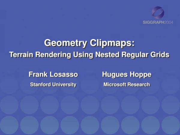
Geometry Clipmaps:Terrain Rendering Using Nested Regular Grids Frank Losasso Stanford University Hugues Hoppe Microsoft Research
Terrain Rendering Challenges Mount Rainier • Concise storage No paging hick-ups • Real-Time frame rates 60 fps • Visual continuity No temporal pops Primary Dataset: United States at 30m spacing20 Billion samples Olympic Mountains
Previous Work • Irregular Meshes (e.g. [Hoppe 98]) • Fewest polygons • Extremely CPU intensive • Bin-trees (e.g. [Lindstrom et al 96]) • Simpler data structures / algorithms • Still CPU intensive • Bin-tree Regions (e.g. [Cignoni et al 03]) • Precomputed regions Decreased CPU cost • Temporal continuity difficult
Previous Work • Texture Clipmaps [Tanner 1998] • ‘Infinitely’ large textures • Clipped mipmap hierarchy • Modeling for the Plausible Emulation of Large Worlds [Dollins 2002] • Quadtree LOD around viewer • Terrain synthesis
Geometry Clipmaps • Store data in uniform 2D grids • Level-of-Detail from nesting of grids • Refine based on distance • Main Advantages • Simplicity • Compression • Synthesis
Terrain as a Pyramid • Terrain as mipmap pyramid • LOD using nested grids Coarsest Level Finest Level
Individual Clipmap Levels • Uniform 2D grid • Indexed triangle strip • Efficient caching • 60 M triangles/second • 255-by-255 grid • Expected Soon: • Vertex Textures
Inter-Level Transitions • Between respective power-of-2 grids
Inter-Level Transitions No transition Geometry transition Geometry & texture transition Gaps in geometry Gaps in texturing/shading
Inter-Level Transitions • Vertex shader blend geometry • Pixel shader blend textures • Both are inexpensive
Clipmap Update • For each level • Calculate new clipmap region • Fill new L-shaped region • Use toroidal arrays for efficiency
Clipmap Update • Update levels coarse-to-fine • Use limited update budget • Only render updated data • Fine levels may be cropped • Rendering load decreases as update load becomes to large for the budget
‘Filling’ New Regions • Two Sources: • Computed on-demand at 60 frames/second Decompressed explicit terrain Synthesized new terrain
Clipmap Update • Fine level from coarse level • U is a 16 point C1 smooth interpolant • For synthesized terrain, X =Gaussian noise • For explicit terrain, X = compression residual
Terrain Synthesis • Adds high frequency detail • Upsample then add Gaussian noise • Precomputed 50-by-50 noise texture • Per-octave amplitude from real terrain
Subdivision Interpolant Bilinear Interpolant (C0) 16-point Interpolant (C1)
Terrain Compression • Create mipmap fine-to-coarse • D found from data such that:
Terrain Compression • Calculate residuals coarse-to-fine • Upsample and compute inter-level residual • Quantize and compress residual • Replace approximation Prevent error accumulation
Compression Results • U.S height map • 30m horizontal spacing • 1m vertical resolution • 216,000-by-93,600 grid • 40GB uncompressed • 350MB compressed factor of over 100 • rms error 1.8m (6% of sample spacing)
Level-of-detail Error • Analyzed statistically See paper • For U.S. terrain (640-by-480 resolution) • rms error = 0.15 pixels • max error = 12 pixels • 99.9th percentile = 0.90 pixels
Graphics Hardware Friendly • Can be implemented in hardware • Clipmap levels as high-precision textures • Subdivision and normal calculation [Losasso et al 03] • Morphing already done in hardware • Noise from Noise() or from texture • Uploaded on-demand • Decompressed terrain
Limitations • Statistical error analysis • Assumes bounded spectral density • Unnecessarily many triangles • Assumes uniformly detailed terrain but, allows for optimal rendering throughput
Advantages • Simplicity • Optimal rendering throughput • Visual continuity • Steady rendering • Graceful degradation • Compression • Synthesis