Download
1 / 39
390 likes | 488 Vues
This introduction explores algebraic reconstruction techniques in longitudinal phase space tomography, utilizing iterative methods for beam distribution reconstruction. Learn about forward and back projections, weight matrices, and tracking maps. Understand the iterative reconstruction process and convergence in reconstructing longitudinal phase space from raw data.

E N D
Introduction to Longitudinal Phase Space Tomography Duncan Scott
Introduction • Integral Transform techniques have been in existence since 1917 • Radon transforms • Iterative, ‘algebraic’ techniques have been developed since the 1970s • Iterative methods are used to reconstruct a beam distribution • They are very simple • Require little input information • Non-linear rotations can be accounted for • Algebraic Reconstruction Techniques Concepts • Forward and Back Projections • Weight Matrix • Tracking Maps • NB the following is qualatitive and for illustration purposes (i.e. minus signs could be wrong).
Forward Projections • Example 2-D density distribution • bunch charge density • Discretized on a grid
Forward Projections (FP) • 2-D density distribution • bunch charge density • Generate Projections, histogram
Forward Projections (FP) • 2-D density distribution • bunch charge density • Generate Projections, histogram • Do at different angles
Mountain Range Plots (Sinogram) • Many projections at different angles give mountain range plot, or sinogram • This is the raw data used to reconstruct the initial density distribution Mountain Range Plot Original Distribution Sinogram
Back Projection (BP) • The contents of a particular projection are evenly shared along all the cells that could have contributed to each bin
Weight Matrix • At arbitrary angles the back/forward projected values can be weighted • e.g. the area the bin intersects with • This will be used in a different way when we consider particles rotating in longitudinal phase space
Iterative Reconstruction • Initial projection data can be quiet crude • 15 bins at 10 angles sinogram • First iteration is an arbitrary guess of the answer • e.g. a grid of zeros • Reconstruction grid can be of any dimension as long as the weight matrix is calculated correctly
Iterative Reconstruction • Forward project the guess for a particular angle and bin FP =0
Iterative Reconstruction • Forward project the guess for a particular angle and bin • The raw data tells us the answer should be 3 FP=0 measurement = 3
Iterative Reconstruction • Forward project the guess for a particular angle and bin • The raw data tells us the answer should be 3 • Back project the difference evenly over contributing cells to give a correction grid ∆cell = 3/15 = 0.2 Weight matrix gives all 1s FP=0 measurement = 3
Iterative Reconstruction • Forward project the guess for a particular angle and bin • The raw data tells us the answer should be 3 • Back project the difference evenly over contributing cells to give a correction grid • Combine the correction grid and the original guess to give the next iteration Guess Correction + = New Guess
Iterative Reconstruction Different shades due to weight matrix • Forward project the guess for a particular angle and bin • The raw data tells us the answer should be 3 • Back project the difference evenly over contributing cells to give a correction grid • Combine the correction grid and the original guess to give the next iteration • Repeat for different projection and Bin
Iterative Reconstruction • Repeat many times and the original image is reconstructed
Convergence - Discrepency • The difference between the measured and reconstructed projections can be used as a merit function for the algorithm • There are numerous, rigorous, demonstrations that iterative algorithms will converge • K. Tanabe, “Projection method for solving a singular system,” Numer. Math. vol. 17, pp. 203-214, 1971.
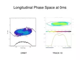
Beam Reconstruction • The above method, with some modifications, can be used to reconstruct the longitudinal phase space of a bunch, given a series of projections from Wall Current Monitors Example raw data from WCM, bunch rotating, aim to reconstruct at injection
Beam Reconstruction 53 MHz, 1MV RF Bucket • The reconstruction grid and projection bins are aligned • The weight matrix contains 1s and 0s • The intersection with the separatrix can slightly change this Bins aligned with reconstruction grid Projection (WCM Signal)
Beam Reconstruction 53 MHz, 1MV RF Bucket • The reconstruction grid and projection bins are aligned • The weight matrix contains 1s and 0s • The intersection with the separatrix can slightly change this • The beam is rotating with variable speed • Account for this by using Tracking Maps to modify the weight matrix Bins aligned with reconstruction grid Projection (WCM Signal)
Tracking Maps • Non-Linear Rotation is accounted for by tracking • Start by Back Projecting a profile
Tracking Maps • Non-Linear Rotation is accounted for by tracking • Start by Back Projecting a profile • Concentrate on one cell • But first a very simple example….
Map Matrix Example • Particle moves from {1,4} to {2,2}
Map Matrix Example • Particle moves from {1,4} to {2,2} • Express grid as a vector • M is the Map
Map Matrix Example • Particle moves from {1,4} to {2,2} • Express grid as a vector • M is the Map
Map Matrix Example • Particle moves from {1,4} to {2,2} • Express grid as a vector • M is the Map • 4th column ‘moves’ particles from 4th component of vector
Map Matrix Example • Particle moves from {1,4} to {2,2} • Express grid as a vector • M is the Map • 4th column ‘moves’ particles from 4th component of vector • Rows determine final position, i.e. 6th
Tracking Maps (cont.) • Non-Linear Rotation is accounted for by tracking • Start by Back Projecting a profile • Concentrate on one cell • We want to know where the particles in this cell were at injection
Tracking Maps (cont.) • Non-Linear Rotation is accounted for by tracking • Start by Back Projecting a profile • Concentrate on one cell • We want to know where the particles in this cell were at injection • Therefore, track backwards
Tracking Maps (cont.) • Non-Linear Rotation is accounted for by tracking • Start by Back Projecting a profile • Concentrate on one cell • We want to know where the particles in this cell were at injection • Therefore, track backwards • After tracking count the number of particles in each cell
Tracking Maps (cont.) • Non-Linear Rotation is accounted for by tracking • Start by Back Projecting a profile • Concentrate on one cell • We want to know where the particles in this cell were at injection • Therefore, track backwards • After tracking count the number of particles in each cell • Doing this for each cell and turn generates a series of maps telling us: what fraction of particles starting in cell X propagate to each other cell in the grid
Example Reconstruction • Back Project 1st profile to give the initial Guess of the answer
Example Reconstruction • Back Project 1st profile to give the initial Guess of the answer • Forward map the Guess a random number of turns
Example Reconstruction • Back Project 1st profile to give the initial Guess of the answer • Forward map the Guess a random number of turns • Project forward- mapped Guess and compare with measurement Measured Answer Difference between Guess and measurement, ∆projection Projection of Forward Mapped Guess
Example Reconstruction • Back Project 1st profile to give the initial Guess of the answer • Forward map the Guess a random number of turns • Project forward mapped Guess and compare with measurement • Back-project ∆projection to create correction grid, ∆grid
Example Reconstruction • Back Project 1st profile to give the initial Guess of the answer • Forward map the Guess a random number of turns • Project forward mapped Guess and compare with measurement • Back project ∆projection to create correction grid, ∆grid • Backward map ∆grid to injection
Example Reconstruction • Back Project 1st profile to give the initial Guess of the answer • Forward map the Guess a random number of turns • Project forward mapped Guess and compare with measurement • Back project ∆projection to create correction grid, ∆grid • Backward map ∆grid to injection • Combine Guess and ∆grid to give new guess and repeat + =
Example Reconstruction • Repeat to reconstruct original beam
Conclusions • Iterative techniques are simple but effective • Compare projections of a Guess to data • Use the comparison to make corrections to Guess • Repeat until difference in projections is suitably small • Maps can be generated using simple or complicated particle tracking and saved • Using saved maps should enable reconstructions to be done “online” • Combined all these elements into ACNET Application • Version 1 goal: • Reconstruct 1 entire batch every 30 seconds • Also get information on single and coupled bunch modes, (beam loading…?) and … ?