Introduction to Tomography
Introduction to Tomography. Presented by Scott Lichtor. Overview. Problem Statement Tomographic Applications The Mathematics Necessary Math Fourier Slice Theorem Filtered Backprojection Matlab Example. Problem. Can’t see inside of people to diagnose problems

Introduction to Tomography
E N D
Presentation Transcript
Introduction to Tomography Presented by Scott Lichtor
Overview • Problem Statement • Tomographic Applications • The Mathematics • Necessary Math • Fourier Slice Theorem • Filtered Backprojection • Matlab Example
Problem • Can’t see inside of people to diagnose problems • Can’t see inside of machinery to diagnose problems • How do take a picture of a place where you can’t fit a camera?
Solution • Tomography • Reconstructs a function using line integrals • Goal: recover the interior structure of a body using exterior measurements • Routine for medicine, earth sciences Image taken from http://media-2.web.britannica.com
Tomography Applications • Single photon emission computed tomography (SPECT) is used for gamma imaging • Gamma-emitting radio-isotope is injected into the body • Gamma camera returns a 2-D image of the object • Reconstruction then returns a 3-D image of the object • Used for medical imaging (tumor imaging, functional brain imaging) Image taken from http://www.biocompresearch.org
Tomography Applications • Positron emission tomography (PET) acquires data from electron-positron annihilation • Positron-emitting tracer is injected into the body • System detects gamma rays produced by tracer • Uses PET to reconstruct 3-D image • Used for oncology, neurology, cardiology, etc. Image taken from http://www.ibfm.cnr.it
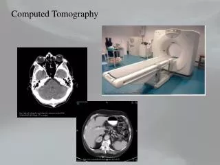
Tomography Applications • Computed tomography (CT) is used for X-ray imaging • X-rays are produced and sent through the body • Record the line integrals • Calculate the shape of the imaged object • Used extensively for medical imaging • Also used for non-destructive materials testing Image taken from http://www.csmc.edu
Tomography • I’ll focus on X-ray tomography • Get interior structure of body by X-raying the object from many different directions • When an X-ray goes through an object, it is attenuated by the object • Very dense objects will weaken the strength of the ray considerable • Less dense objects will affect the strength of the ray less
History of Computed Tomography • Alessandro Vallebona proposed representing a slice of the body on radiographic film in the early 1900s • First commercially viable CT scanner invented by Sir Godfrey Hounsfield at EMI Laboratories in 1972 • Originally, water tanks were needed for imaging on humans
Necessary Mathematics • Line integrals are integrals along a line • Coordinate system: (x,y)->(Ѳ,t) • Ѳ: Angle, t: distance along source • Fourier Transform: F(w) = ∫f(t)e-j2πwtdt • F(u,v)=∫∫f(x,y)e-j2π(ux+vy)dxdy Image taken from http://www.mindef.gov.sg
Tomography • A projection is composed of a bunch of line integrals • Easiest example: line integrals with the same Ѳ but different t’s (parallel line integrals). • The value of a line integral: • PѲ(t) = ∫(Ѳ,t)line f(x,y)ds • PѲ(t) = ∫∫f(x,y)δ(x cos(Ѳ)+y sin(Ѳ)-t)dxdy • Radon transform
Fourier Slice Theorem • Object function is f • Fourier transform of f is F • Projection P • Fourier transform of P is S • F(u,v)=∫∫f(x,y)e-j2π(ux+vy)dxdy • SѲ(w) = ∫PѲ(t)e-j2πwtdt • To demonstrate the Fourier Slice Theorem, let Ѳ=0
Fourier Slice Theorem • Suppose v=0 • F(u,0) = ∫∫f(x,y)e-j2πuxdxdy • = ∫(∫f(x,y)dy)e-j2πuxdx • PѲ=0(x) = ∫ f(x,y)dy • So F(u,0) = ∫ PѲ=0(x) e-j2πuxdx • There’s a relationship between the projection data and the object image • Specifically, each projection gives a slice of the Fourier transform of the overall image Image taken from http://www.eng.warwick.ac.uk
Filtered Backprojection • Filtered backprojection is the algorithm used to reconstruct the object image • Idea: use the projection data to get slices of the Fourier transform of the object image. Then, calculate the object image Image taken from http://www.eng.warwick.ac.uk
Filtered Backprojection • Procedure: For all angles K 1. Get projections P Ѳ 2. Apply Fourier transform and get SѲ(w) 3. Place the inverse Fourier transforms of the projections on the approximation of the original image In this way an approximation of the original image can be obtained (this is only the algorithm for parallel projections)
Example • Matlab illustration • Typical image to reconstruct:
Example • Create projection data • Use the radon function • The radon function applies the radon transform to an image
Example • 18 projections
Example • 36 projections
Example • 90 projections
Example • The imradon function reconstructs images from projection data
Example • Reconstruction with 36 projections
Example • Reconstruction with 36 projections
Example • Reconstruction with 90 projections
Sources • An Introduction to X-ray tomography and Radon Transforms, by Eric Todd Quinto • Principles of Computerized Tomographic Imaging, by Avinash C. Kak and Malcolm Slaney • Wikipedia