Analyzing Prices vs. Quantities: Insights from Baumol and Oates

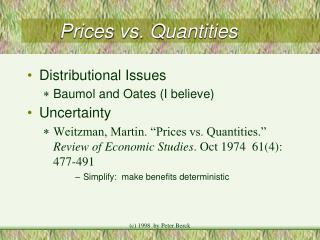
1. Prices vs. Quantities • Distributional Issues • Baumol and Oates (I believe) • Uncertainty • Weitzman, Martin. “Prices vs. Quantities.” Review of Economic Studies. Oct 1974 61(4): 477-491 • Simplify: make benefits deterministic (c) 1998 by Peter Berck

2. Before regulation profits are dark green and purple areas When regulation reduces Q Profits are the purple plus green areas (mcf > mr as drawn) Tax mc If, instead, tax T=mc-mcf at reg Q: Q is still Reg Q, green area is tax take and only purple remains as profit mcf mcp Unreg. Q Reg Q

3. The Uncertainty Problem • A private producer needs to be motivated to produce a good that is not sold in a market. • The government does not know the costs of producing the goods. • In particular it does not know a, a mean zero variance 2element of the cost function

4. Quantity Regulation • The firm can be told to produce a quantity certain, qr. • The level of benefits will be certain, since qr is certain, but • the level of costs isn’t known so the government will accept the uncertainty in the cost to be paid.

5. Price Motivation • Or, the Government can offer to pay a price, p for any units produced. • The firm will observe which cost they incur and react to the the true supply curve and set p=mc correctly, • but the level of production and level of benefits will be variable

6. Which to choose? • Professor Weitzman (to the best of my ancient memory) gave the example of medicine to be delivered to wartime Nicaragua. • Too little and people die • Too much not worth anything more • cost doesn’t matter that much • so, choose qr and get the right amount there for certain

7. In quantity mode, • the regulator chooses a quantity, qr, • then the state of nature becomes known, • then the firm produces and costs are incurred and benefits received. • B(q) is benefits and B’ is marginal benefit. • C(q,a) is cost and is a function of the state of nature, a.

8. B’ = MC • qr = argmaxq E( B - C). • Gives the optimal choice of qr. • Of course, E[B’ - Cq] = 0 at qr.

9. Approximate About qr • Approximate B and C about qr. • Note that the uncertainty in marginal cost is all in a, which is just a parallel shift in mc. Could also have a change in slope. • C(q,a) = c +( c’ + a) (q-qr) + .5 c’’ (q-qr)2 • B(q) =b + b’ (q-qr) + .5 b’’ (q-qr)2 • b and c are benefits and costs at qr

10. Obvious algebra. • mc = c’ + a+ c’’ (q-qr) • marginal cost • E[mc(qr,a)] = c’ + E[a] = c’ • mb = b’ + b’’ (q- qr) • marginal benefit • E[B’(qr) ] = b’ • FOC for qr implies b’=c’

11. B’ A picture. • mc = c’ + a+ c’’ (q-qr); here a takes on the values of • +/- e with equal probability • . qr c’+e + c’’ (q-qr) c’-e + c’’ (q-qr) c’ + c’’ (q-qr)

12. B’ As the slope of B’ approaches vertical DWL goes down Deadweight Loss using qr. +e Half the time each triangle is the DWL -e qr

13. The Supply Curve • The firm sees the price, p, and maximizes its profits after it knows a, so • p = mc • p = c’ + a + c’’ (q-qr) • Solving gives the supply curve: • h(p,a) = q = qr + (p - c’ - a) / c’’

14. The center chooses p … • The center chooses p to maximize expected net benefits: • p* = argmaxp E[ B(h(p,a) - C(h(p,a))] • B-C = b-c +(b’-c’- a)(q-qr) + (b’’-c’’).5(q-qr)2 • substitute q-qr = (p - c’ - a) / c’’ • = b-c - a(p - c’ - a) / c’’ • + (b’’-c’’).5 ((p - c’ - a) / c’’ )2 • Zero by FOC for qr

15. Take Expectations • B-C = b-c - a(p - c’ - a) / c’’ • + (b’’-c’’).5 ((p - c’ - a) / c’’ )2 • E[B-C] = b-c + 2/c” + • (b’’-c’’) {(p-c’)2 + 2}/ {2c”2} • 0 = DpE[B-C] = p - c’ • E[B-C] • = b-c + 2/c” + {(b’’-c’’)2}/ {2c”2}

16. Advantage of Prices over Quant. • Under price setting • E[B-C] • = b-c + 2/c” + {(b’’-c’’)2}/ {2c”2} • Less E[B-C] under quantity: = b-c • Advantage of price over quantity….

17. The advantage of prices over quantities

18. As the slope of B’ approaches vertical DWL goes up B’ Deadweight Loss using p*. +e Half the time each triangle is the DWL -e P*