Download
1 / 50
520 likes | 717 Vues
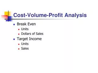
Cost-Volume-Profit Analysis. Identify different cost behavior patterns. Objective 1. Types of Costs. Variable. Fixed. Mixed. Variable Costs Example. Consider Grand Canyon Railway. Assume that breakfast costs Grand Canyon Railway $3 per person.

E N D
Identify different cost behavior patterns. Objective 1
Types of Costs Variable Fixed Mixed
Variable Costs Example • Consider Grand Canyon Railway. • Assume that breakfast costs Grand Canyon Railway $3 per person. • If the railroad carries 2,000 passengers, it will spend $6,000 for breakfast services.
Variable Costs Example Total Variable Costs (thousands) $24 – $18 – $12 – $6 – – – – – 0 1 2 3 4 5 Volume (Thousands of passengers)
Fixed Costs Example $400 – $300 – $200 – $100 – Total Fixed Costs (thousands) – – – – 0 1 2 3 4 5 Volume (Thousands of passengers)
Mixed Costs Example • A mixed cost is part variable and part fixed. • Assume a department of a company has fixed costs of $50 per month ($600 per year). • There are also variable costs of $3 per hour.
Mixed Costs Example $2,850 – $2,100 – $1,350 – $600 – Total Costs Variable Cost – – – – Fixed Cost 0 125 250 375 500 625 Volume (hours)
Relevant Range... • is a band of volume in which a specific relationship exists between cost and volume. • Outside the relevant range, the cost either increases or decreases. • A fixed cost is fixed only within a given relevant range and a given time span.
Relevant Range $160,000 – $120,000 – $80,000 – $40,000 – – – Fixed Costs Relevant Range 0 5,000 10,000 15,000 20,000 25,000 Volume in Units
Use a contribution margin income statement to make business decisions. Objective 2
Two Approaches to Compute Profits Conventional income statement Contribution margin income statement
Conventional Income Statement Sales Cost of Goods Sold Gross Margin – = Net Income Gross Margin Operating Expenses – =
Contribution MarginIncome Statement Sales Variable Expenses Contribution Margin – = Net Income Contribution Margin Fixed Expenses – =
Contribution Margin Example • Luis and Tom manufacture a device that allows users to take a closer look at icebergs from a ship. • The usual price for the device is $100. • Variable costs are $70. • They receive a proposal from a company in Newfoundland to sell 20,000 units at a price of $85.
Contribution Margin Example • There is sufficient capacity to produce the order. • How do we analyze this situation? • $85 – $70 = $15 contribution margin. • $15 × 20,000 units = $300,000 (total increase in contribution margin)
Compute breakeven sales and perform sensitivity analyses. Objective 3
Cost-Volume-Profit Analysis — Sales — Fixed — Fixed + Variable
Cost-Volume-Profit Analysis • Accountants use two methods to perform CVP analysis. • Both methods use an equation or formula derived from the contribution margin income statement. Sx – Vx – F = 0
Equation Approach With the equation approach, breakeven sales in units is calculated as follows: Unit sales price × Units sold – Variable unit cost × Units sold – Fixed expenses = Operating income
Breakeven Point Example • Assume that fixed expenses amount to $90,000. • How many devices must be sold at the regular price of $100 to break even? • ($100 × Units sold) – ($70 × Units sold) – $90,000 = 0 • Units sold = $90,000 ÷ $30 = 3,000
Contribution Margin Per Unit Percent Ratio Sales price $100 100 1.00 Variable expenses 70 70 .70 Contribution margin $ 30 30 .30
Contribution Margin Formula (Fixed expenses + Operating income) ÷ Contribution margin per unit = Units ($90,000 + 0) ÷ $30 = 3,000 Units
Contribution Margin Ratio Formula (Fixed expenses + Operating income) ÷ Contribution margin ratio = $ Sales ($90,000 + 0) ÷ .30 = $300,000
Change in Sales Price Example • Suppose that the sales price per device is $106 rather than $100. • What is the revised breakeven sales in units? • New contribution margin: $106 – $70 = $36 • $90,000 ÷ $36 = 2,500 units
Change in Variable Costs Example • Suppose that variable expenses per device are $75 instead of $70. • Other factors remain unchanged. • $90,000 ÷ $25 = 3,600 • $90,000 ÷ 0.25 = $360,000
Change in Fixed Costs Example • Suppose that rental costs increased by $30,000. • What are the new fixed costs? • $90,000 + $30,000 = $120,000 • What is the new breakeven point? • $120,000 ÷ $30 = 4,000 units • $120,000 ÷ 0.30 = $400,000
Compute the sales level needed to earn a target operating income. Objective 4
Target Operating Income Example • Suppose that a business would be content with operating income of $45,000. • Assuming $100 per unit selling price, variable expenses of $70 per unit, and fixed expenses of $90,000, how many units must be sold? • ($90,000 + $45,000) ÷ $30 = 4,500
Graph a set of cost-volume-profit relationships. Objective 5
Various Sales Levels Example • Assume selling price is $35 per unit. • Variable expense is $21 per unit. • Fixed cost is $7,000. • What is the breakeven point? • 500 units or $17,500
Cost-Volume-Profit Graph Breakeven sales point 500 units or $17,500 Sales revenue line Total expense line Fixed expense line
Various Sales Levels Example • What operating income is expected when sales are 300 units? • $14 × 300 = $4,200 $4,200 – $7,000 = ($2,800)
Various Sales Levels Example • What operating income is expected when sales are 1,000 units? • $14 × 1,000 = $14,000 $14,000 – $7,000 = $7,000
Compute a margin of safety. Objective 6
Margin of Safety Example • Margin of safety is the excess of expected sales over breakeven sales. • Assume Luis and Tom’s breakeven point is 3,000 devices. • Suppose they expect to sell 4,000 during the period. • What is the margin of safety?
Margin of Safety Example 4,000 – 3,000 = 1,000 units 1,000 × $100 = $100,000 1,000 × 4,000 = 25% $100,000 × $400,000 = 25%
Assumptions of CVP Analysis • Expenses can be classified as either variable or fixed. • CVP relationships are linear over a wide range of production and sales. • Sales prices, unit variable cost, and total fixed expenses will not vary within the relevant range.
Assumptions of CVP Analysis • Volume is the only cost driver. • The relevant range of volume is specified. • Inventory levels will be unchanged. • The sales mix remains unchanged during the period.
Use the sales mix in CVP analysis. Objective 7
Sales Mix Example • Suppose that Luis and Tom plan to sell two types of devices instead of one. • They estimate that sales will be 3,000 regular devices and 1,000 large devices. • This is a 3:1 sales mix. • They expect 3/4 of the devices sold to be regular devices and 1/4 to be large devices.
Sales Mix Example RegularLarge Sales price $100 $154 Variable expenses 70 100 Contribution margin 30 54 Sales mix (units) 3 1 $ 90 $ 54 The total is $144.
Sales Mix Example Weighted-average contribution margin $144 ÷ (3 + 1) = $36 Breakeven sales $90,000 ÷ $36 = 2,500 2,500 × 3/4 = 1,875 regular devices 2,500 × 1/4 = 625 large devices
Sales Mix Example 1,875 regular × $100 = $187,500 625 large × $154 = 96,250 Breakeven $283,750 $90,000 ÷ $144 = 625 packages in the mix
Compute income using variable costing and absorption costing. Objective 8
Product Costing Absorption costing assigns all manufacturing costs to products. Financial statements prepared under GAAP use absorption costing. Variable costing assigns only variable manufacturing costs to products. Variable costing is for internal use only.
Product Costing Example Assume the following costs: Direct material unit cost $6.00 Direct labor unit cost $3.00 Variable manufacturing overhead $2.00 Variable marketing $2.50 Fixed manufacturing overhead per unit $5.00 What is the product cost/unit?
Product Costing Example Absorption Costing Direct materials $ 6.00 Direct labor 3.00 Variable manufacturing overhead 2.00 Fixed manufacturing overhead 5.00 Total $16.00
Product Costing Example Variable Costing Direct materials $ 6.00 Direct labor 3.00 Variable manufacturing overhead 2.00 Fixed manufacturing overhead -0- Total $11.00