Download
1 / 41
410 likes | 614 Vues
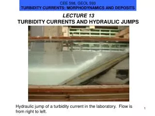
CEE 598, GEOL 593 TURBIDITY CURRENTS: MORPHODYNAMICS AND DEPOSITS. LECTURE 10 SELF-ACCELERATION OF TURBIDITY CURRENTS. Let’s compare the momentum equation for a river and a turbidity current: River: Turbidity current.

E N D
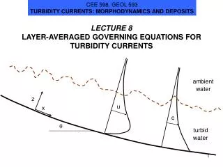
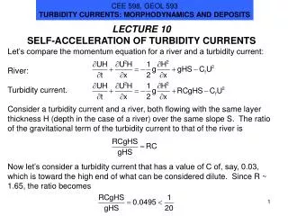
CEE 598, GEOL 593 TURBIDITY CURRENTS: MORPHODYNAMICS AND DEPOSITS LECTURE 10 SELF-ACCELERATION OF TURBIDITY CURRENTS Let’s compare the momentum equation for a river and a turbidity current: River: Turbidity current. Consider a turbidity current and a river, both flowing with the same layer thickness H (depth in the case of a river) over the same slope S. The ratio of the gravitational term of the turbidity current to that of the river is Now let’s consider a turbidity current that has a value of C of, say, 0.03, which is toward the high end of what can be considered dilute. Since R ~ 1.65, the ratio becomes
THE INHERENTLY WEAK DRIVING OF TURBIDITY CURRENTS COMPARED TO RIVERS For the example considered, then, Now we know that rivers can excavate deep submarine canyons, such as the Grand Canyon to the left. If turbidity currents have such weak driving, how can they excavate canyons?
THE INHERENTLY WEAK DRIVING OF TURBIDITY CURRENTS COMPARED TO RIVERS contd. How do they do it?
THE SLOPE EFFECT One way turbidity currents can be made stronger is by jacking up the bed slope. Let Sf denote the fluvial bed slope and St denote the slope of the turbidity current channel. Again considering the case of the same flow thickness H for both cases, the ratio of the driving forces is now Thus if the following relation holds: a turbidity current has the same driving force as a river. For example, for the example of the previous slides, And indeed, the slopes of both canyons and fan channels associated with turbidity currents tend to be steeper than rivers of otherwise similar dimensions.
LET’S LOOK AT THE AMAZON CANYON/FAN SYSTEM Pirmez (1994)
LONG PROFILE OF THE AMAZON SUBAERIAL/SUBMARINE SYSTEM Note that the submarine slopes are much higher than the subaerial slopes. Pirmez and Imran, (2003)
MORE DETAILS OF THE LONG PROFILE OF THE AMAZON SUBMARINE CANYON-FAN SYSTEM Amazondata.xls
ELEVATION AND SLOPE PROFILES OF THE AMAZON SUBMARINE CANYON-FAN SYSTEM
DEPTH VERSUS SLOPE: AMAZON SUBMARINE CHANNEL VERSUS SOME OF THE LARGEST RIVERS IN THE WORLD The river depths are the depths at bankfull flow. The turbidity current channel depths are thalweg (deepest point) to levee crest depths, which exaggerates the depth somewhat (by a factor of about 1.5?) Yes, the slopes for the turbidity current channel are much steeper!
BUT THERE IS ANOTHER WAY TO MAKE STRONG TURBIDITY CURRENTS: SELF-ACCELERATION Start them small And grow them large!
CONSIDER THE FORMATION OF SNOW DONUTS “According to Mike Stanford from our WSDOT avalanche team, snow doughnuts are a natural occurrence in nature. We do not build them. They form when there is a hard layer in the snow and is then covered by several inches of dense snow. Then you add a steep slope and a trigger, such as a clump of snow falling out of a tree or off of a rock face, and voila you have snow doughnuts. “ http://www.wsdot.wa.gov/traffic/passes/northcascades/2007/pictures
SNOW DONUTS AS A CONCEPTUAL EXAMPLE OF SELF-ACCELERATION “Snow doughnuts seemingly could grow very big if conditions permitted. The one seen in the photograph is about 24" in diameter.” http://www.wsdot.wa.gov/traffic/passes/northcascades/2007/pictures • For some reason, a small ball (or donut) of snow starts rolling down a hill. If the hill is steep enough (and the snow is of the right stickiness), • gravity accelerates the ball, which then gathers more snow as it roll, • which makes it heavier, • which makes it go even faster in a self-reinforcing cycle. • The snowball eventually decelerates and comes to rest when it reaches the base of the slope. • This is a way to make a big snowball out of an initially small snowball! • Start it small, grow it big! See also Fukushima and Parker (1990)
THE POSSIBILITY OF OF SELF-ACCELERATION (“IGNITION”) AND SELF-DECELERATION OF A TURBIDITY CURRENT Consider the 3-equation model. We write Es = Es(U) to indicate that it is a function of velocity. Pantin (1979); Parker (1982); Fukushima et al. (1985); Parker et al. (1986) • Start off with a “small” (but not too “small”) current. • The combination of initial (or upstream) U and C is just right so Es < roC. • The concentration of sediment C thus increases. • As a result, the flow gets heavier. • Because it is heavier, it accelerates and increases U • Increased U leads to increased Es. • Go back to step 2 and repeat. • The same process can lead to self-deceleration if the current is too “small”.
A SIMPLIFIED CONCEPTUAL MODEL Here m is a free parameter. Note that the equations have an equilibrium (fixed point) at (U, C) = (1, 1).
A SIMPLIFIED CONCEPTUAL MODEL contd. We can solve these equations subject to initial conditions. For example, define t1 = 0, ti+1 = ti + t where t is a time step, and Ui and Ci denote the values of U and C at ti. Using the simple Euler step method, U, C This gives us curves like t
initial condition Fixed point PHASE DIAGRAM The solution can be represented in terms of a phase diagram in which C is plotted against U. In the case conceptually illustrated below, the current eventually goes into self-acceleration, with U and C both increasing.
CASE: m < 2 In this case the equation set is stable, and the flow converges to the fixed point (U, C) = (1, 1) for any initial condition. Here the case (Uinit , Cinit) = (1.1, 0.2) is illustrated for m = 1.7. The calculation was performed with IgnitPlotTurbCurr.xls
CASE: m > 2: SELF-ACCELERATION In this case the equation set is unstable, and the flow diverges away from the fixed point (self-acceleration or self-deceleration) for any initial condition for which (Uinit, Cinit) (1, 1). The case below, which illustrates self-acceleration is for the case (Uinit, Cinit) = (1.3, 0.75) and m = 2.5.
CASE: m > 2: SELF-DECELERATION The case below illustrates self-deceleration for the case (Uinit, Cinit) = (1.3, 0.6) and m = 2.5.
REGIME DIAGRAM For any case m > 2, it is possible to determine a regime diagram that a) divides the self-accelerating regimes from the self-decelerating regime, and b) shows a line to which the solution eventually converges for any initial condition.
TURBIDITY CURRENTS WITH THE 3-EQUATION MODEL This time we consider flows that are steady in time but developing in the downstream direction. The calculations are performed with the 3-equatoin model: The upstream boundary conditions are A necessary condition for solving the flow downstream is that the initial flow be supercritical, i.e. Rio = (Rgqs/U3)o < 1. (This does not mean that subcritical flows cannot be treated. They require, however, integration in the upstream rather than downstream direction.
SAMPLE CALCULATION: SELF-ACCELERATION The 3-equation model does not have a fixed point (equilibrium corresponding to normal flow). This notwithstanding, both self-accelerating and self-decelerating regimes can be defined. The example below shows the calculation conditions for an example generated with TurbCurrSpatIg3equ.xls
RESULTS: SELF-ACCELERATION Note that both U and qs increase downstream. U reaches a very high value of ~ 8 m/s 4000 m downstream of the starting point. The bed slope is 0.03.
RESULTS: SELF-DECELERATION The calculation conditions are exactly the same as those of the previous slide, except that the bed slope is lowered to 0.02.
TURBIDITY CURRENTS WITH THE 4-EQUATION MODEL The governing equations are: and the upstream initial conditions are specified as:
SAMPLE CALCULATION WITH THE 4-EQUATION MODEL The calculation conditions correspond to the example of self-acceleration fiver for the 3- equation model. The calculation is performed using TurbCurrSpatIg4equ.xls.
STRATIFICATION EFFECTS CHANGE THE NATURE OF THE SOLUTION The effect of damping of the turbulence due to stratification effects in the 4-equation model pushes this case into the regime of self-deceleration.
SELF-ACCELERATION WITH THE 4-EQUATION MODEL If the slope S is increased to 0.075, the flow does go into self-acceleration. But the velocity realized 4 km downstream is much less than the case using the 3-equation model presented earlier. The inclusion of stratification effects still allow for self-acceleration, but the conditions are more stringent.
EXCAVATION OF SUBMARINE CANYONS Self-acceleration is a way by which a relatively small flow, generated by any condition such as breaching, hyperpycnal flow, retrogressive delta failure, or wave action, can generate a current strong enough to excavate submarine canyons. Xu, Noble, Rosenfeld, Paull (USGS, NPS, MBARI)
WHEN THE CALCULATION FAILS Under some conditions, the calculation fails at some point downstream. There are various reasons for this (e.g. time step too large), but among them is an important physical reason. Consider the example input shown below for the 3-equation model. The calculation is supposed to be performed out to x = 0.25 x 1000 = 250 m.
WHEN THE CALCULATION FAILS contd. The numerical model fails at x = 110 m, well short of the intended distance of x = 250 m
WHAT HAPPENED? Note that the Richardson number Ri rises to 1 at x = 110 m. This implies that there must be a hydraulic jump to subcritical flow upstream of this point, because the bed slope is too low to support the flow. The precise location of the hydraulic jump is determined by dowstream conditions. Its location must be determined by upstream integration of the ‘backwater’ equations from a control point downstream. hydraulic jump H
IN A SUBMARINE CANYON-FAN SYSTEM, THE DECLINE IN SLOPE DOWNSTREAM CAN CAUSE A HYDRAULIC JUMP This jump can often be associated with the transition from the canyon to the fan. Recall that subcritical flow has a very low entrainment entrainment rate of ambient water. This can allow the flow to stay more or less confined within a leveed channel. Hydraulic jump?
EVIDENCE FOR THE HYDRAULIC JUMP The 4-equation model applied to an erodible bed indicates the formation of sediment waves in the vicinity of the hydraulic jump. (More about this will be presented in a subsequent chapter.) A sample calculation is shown below. Kostic and Parker (2006)
CANYON-FAN TRANSITION ON THE NIGER MARGIN Let’s look here From Prather and Pirmez (2003)
THE SEDIMENT WAVES sediment waves
LIMITS TO SELF-ACCELERATION • Self-acceleration cannot occur indefinitely. The following factors limit it. • Declining slope downstream must eventually move the flow out of the self-acceleration regime. • Under some conditions, it appears that strong stratification effects near slope breaks can turn off the turbulence and kill the flow. • Even in a submarine canyon of sufficient steepness to support continued self-acceleration, at some point the bed is eroded to bedrock (stiff, consolidated clay in many submarine canyons), and so no more sediment can be entrained (except for that supplied by a slow rate of bed incision). • Such conditions are called “bypass” conditions. The sediment load is simply transferred downstream without erosion or deposition, so that the suspended sediment load becomes constant. In a canyon of constant width, then, whatever settles is immediately entrained without further bed erosion, and
qs u qs bed swept clean to bedrock BYPASS CONDITIONS AND EXCAVATION OF SUBMARINE CANYONS incision The passage of repeated turbidity currents that are powerful enough to reach bypass conditions can (one flow at a time) slowly cause channel incision, leading to the formation of the canyon. Canyon incision cannot occur until the bed is swept clean of easily erodible sediment.
SELF-ACCELERATION DOES NOT APPLY ONLY TO FLOWS THAT ARE STEADY IN TIME AND DEVELOPING IN SPACE The calculation uses the 4-equation model retaining the time terms. It shows how a small pulse-like flow can self-accelerate into a long, quasi-continuous flow on a steep slope, and then decelerate on a lower slope (0 in this case). Pratson et al. (2001)
REFERENCES Fukushima, Y., Parker, G. and Pantin, H., 1985, Prediction of igniting turbidity currents in Scripps Submarine Canyon. Marine Geology, 67, 55-81. Fukushima, Y. and Parker, G., 1990, Numerical simulation of powder snow avalanches. Y. Fukushima and G. Parker, Journal of Glaciology, 36(2), 229 237. Kostic, S. and Parker, G., 2006, The response of turbidity currents to a canyon-fan transition: internal hydraulic jumps and depositional signatures, Journal of Hydraulic Research, 44(5) 631–653. Pantin, H. M., 1979, Interaction between velocity and effective density in turbidity flow: phase-plane analysis, with criteria for autosuspension, Marine Geology, 31, 59-99. Parker, G., 1982, Conditions for the ignition of catastrophically erosive turbidity currents. Marine Geology, 46, pp. 307‑327, 1982. Parker, G., Y. Fukushima, and H. M. Pantin, 1986, Self‑accelerating turbidity currents. Journal of Fluid Mechanics, 171, 45‑181. Parker, G., M. H. Garcia, Y. Fukushima, and W. Yu, 1987, Experiments on turbidity currents over an erodible bed., Journal of Hydraulic Research, 25(1), 123‑147. Pirmez, C., 1994, Growth of a submarine meandering channel–levee system on Amazon Fan, PhD Thesis, Columbia University, New York, 587 p. Pirmez, C. and Imran, J., 2003, Reconstruction of turbidity currents in a meandering submarine channel, Marine and Petroleum Geology 20(6-8), 823-849. Prather, B. E. and Pirmez, C., 2003 Evolution of a shallow ponded basin, Niger Delta slope, Annual Meeting Expanded Abstracts, American Association of Petroleum Geologists, 12, 140-141. Pratson, L. F, Imran, J, Hutton, E.W.H., Parker, G. and Syvitski, J.P.M., 2001, Debris Flows vs. Turbidity Currents: a Modeling Comparison of Their Dynamics and Deposit, Computers & Geosciences 27, 701–716.