Fracture/Conduit Flow
Fracture/Conduit Flow. Fractured rock (NSW Australia). Motivation. Karst. http://research.gg.uwyo.edu/kincaid/Modeling/wakulla/wakcave2.jpg. ~11 m 3 s -1. ~100 m. White Scar, England; photo by Ian McKenzie, Calgary, Canada.

Fracture/Conduit Flow
E N D
Presentation Transcript
Fractured rock (NSW Australia) Motivation
Karst http://research.gg.uwyo.edu/kincaid/Modeling/wakulla/wakcave2.jpg ~11 m3 s-1 ~100 m White Scar, England; photo by Ian McKenzie, Calgary, Canada
These data and images were produced at the High-Resolution X-ray Computed Tomography Facility of the University of Texas at Austin
Momentum • p = mu
Viscosity • Resistance to flow; momentum diffusion • Low viscosity: Air • High viscosity: Honey • Kinematic viscosity:
Reynolds Number • The Reynolds Number (Re) is a non-dimensional number that reflects the balance between viscous and inertial forces and hence relates to flow instability (i.e., the onset of turbulence) • Re = v L/n • L is a characteristic length in the system • Dominance of viscous force leads to laminar flow (low velocity, high viscosity, confined fluid) • Dominance of inertial force leads to turbulent flow (high velocity, low viscosity, unconfined fluid)
Re << 1 (Stokes Flow) Tritton, D.J. Physical Fluid Dynamics, 2nd Ed. Oxford University Press, Oxford. 519 pp.
Re = 30 Re = 40 Re = 47 Re = 55 Re = 67 Re = 100 Eddies, Cylinder Wakes, Vortex Streets Tritton, D.J. Physical Fluid Dynamics, 2nd Ed. Oxford University Press, Oxford. 519 pp. Re = 41
Eddies and Cylinder Wakes S.Gokaltun Florida International University Streamlines for flow around a circular cylinder at 9 ≤ Re ≤ 10.(g=0.00001, L=300 lu, D=100 lu)
Eddies and Cylinder Wakes S.Gokaltun Florida International University Streamlines for flow around a circular cylinder at 40 ≤ Re ≤ 50.(g=0.0001, L=300 lu, D=100 lu) (Photograph by Sadatoshi Taneda. Taneda 1956a, J. Phys. Soc. Jpn., 11, 302-307.)
Poiseuille Flow z u Flow y a x L
Poiseuille Flow • In a slit or pipe, the velocities at the walls are 0 (no-slip boundaries) and the velocity reaches its maximum in the middle • The velocity profile in a slit is parabolic and given by: u(x) • G can be due to gravitational acceleration (G = rg in a vertical slit) or the linear pressure gradient (Pin – Pout)/L x = 0 x = a/2
Poiseuille Flow • Maximum • Average u(x) x = 0 x = a/2
Poiseuille Flow S.GOKALTUN Florida International University
I1 I2 I3 Kirchoff’s Current Law • Kirchoff’s law states that the total current flowing into a junction is equal to the total current leaving the junction. node Gustav Kirchoff was an 18th century German mathematician I1flowsintothe node I2flowsoutof the node I1= I2+ I3 I3flowsoutof the node
Ohm’s law relates the flow of current to the electrical resistance and the voltage drop • V = IR (or I = V/R) where: • I = Current • V = Voltage drop • R = Resistance • Ohm’s Law is analogous to Darcy’s law
Poiseuille's law can related to Darcy’s law and subsequently to Ohm's law for electrical circuits. • Cubic law: A = a *unit depth
36 lu DP12 Q12 900 lu Q23 DP23 54 lu Q34 DP DP34 108 lu Q45 DP45 Q56 DP56 -216 lu - Fracture Network
Back Solution • Have conductivities and, from the matrix solution, the gradients • Compute flows • Also have end pressures • Compute intermediate pressures from DPs
Q (lu3/ts) Re LBM Kirchoff’s 0.66 0.11 0.11 1.0 0.14 0.14 1.8 0.18 0.19 4.1 0.27 0.28 7.2 0.36 0.37 43.0 0.87 0.92 Hydrologic-Electric Analogy Poiseuille's law corresponds to theKirchoff/Ohm’s Lawfor electrical circuits, where pressure drop Δp is replaced by voltage V and flow rate by current I a I12 ΔP12 I23 I23 ΔP23 I34 ΔP34 I45 ΔP45 I45 I56 ΔP56 Q = 0.11 lu3/ts Q = 0.11 lu3/ts Kirchoff LBM
Entry Length Effects Tritton, D.J. Physical Fluid Dynamics, 2nd Ed. Oxford University Press, Oxford. 519 pp.
Eddies Serpa, CY, 2005, Unpublished MS Thesis, FIU Bai, T., and Gross, M.R., 1999, J Geophysical Res, 104, 1163-1177 2 mm 3 mm 3.3 mm x 2.7 mm Re = 9 Flow
‘High’ Reynolds Number Taneda, J. Fluid Mech. 1956. (Also Katachi Society web pages) • Single cylinder, Re ≈ 41
Darcy-Forschheimer Equation • Darcy: • +Non-linear drag term:
Apparent K as a function of hydraulic gradient • Gradients could be higher locally • Expect leveling at higher gradient? t = 1 Darcy-Forchheimer Equation
Streamlines at different Reynolds Numbers Re = 152 K = 20 m/s Re = 0.31 K = 34 m/s • Streamlines traced forward and backwards from eddy locations and hence begin and end at different locations
Future • Gray scale as hydraulic conductivity, turbulence, solutes