Improving Pulsar Timing
Willem van Straten George Hobbs, Rick Jenet. Improving Pulsar Timing. Why?. Gravitational Wave detection/sensitivity MSPs binary system dynamics Astrometry: Solar System Ephemeris Earth Wobble Terrestrial Time Timing Noise (incl. glitches). G. Hobbs. Software/Modeling. How?.

Improving Pulsar Timing
E N D
Presentation Transcript
Willem van Straten George Hobbs, Rick Jenet Improving Pulsar Timing
Why? • Gravitational Wave detection/sensitivity • MSPs binary system dynamics • Astrometry: • Solar System Ephemeris • Earth Wobble • Terrestrial Time • Timing Noise (incl. glitches)
Software/Modeling How? Numerical Precision Arrival Time Estimation • Precision (Noise) Time Standard Polarimetric Calibration Interstellar Scintillation Earth Wobble Accuracy (Systematics) RFI Mitigation Solar System Ephemeris Solar Wind Earth Atmosphere DM Variation Clock Correction Time/Freq Resolution Sensitivity Hardware/Instrumentation
Modelling Software (tempo2) • Clock Corrections • Physical Delays: • Solar System Ephemeris (incl. Shapiro delay) • Earth Wobble precession & nutation (40ns) polar motion (60ns) • Atmospheric Delays troposphere (20ns) ionosphere (1ns)
RFI mitigation using an adaptive filter Kesteven et al. (2004)
Interstellar Scintillation Figure 1, Walker & Stinebring (2005)
Arrival Time Estimation • Frequency domain (Taylor 1992) • Multi-component Gaussian (Kramer et al. 1994) • Invariant interval (Britton et al. 2000) • Full polarization (van Straten 2004) • Time vs. frequency domain (Hotan et al. 2005) • Higher order moments (Jenet & Hobbs 2005)
Full Polarization TOA • Stokes Q, U, V often sharper than Stokes I • Useful for timing? (Kramer et al. 1999)
Formalism van Straten (2004)
Simulation Position Angle of Linear Polarization: Gaussian Total Intensity Profile with Width, w Constant Degree of Polarization, p Measurement noise, n
PSR J0437-4715 1.1
PSR J1713+0747 1.0
PSR B1937+21 1.4
PSR J1022+1001 1.6
Conclusion • Full Polarization TOA holds promise • Effectiveness varies by pulsar • To do: • Produce/acquire well-calibrated, high S/N polarimetric pulse profile (standards) • Run simulations • Improve arrival time estimates