Agenda

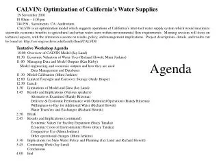
1. CALVIN: Optimization of California’s Water Supplies  29 November 2001 10:00am – 4:00 pm 744 P St., Sacramento, CA; Auditorium  CALVIN is an optimization model which suggests operations of California’s inter-tied water supply system which would maximize statewide economic benefits to agricultural and urban water users within environmental flow requirements. Morning sessions will focus on technical aspects, with the afternoon sessions on results, policy, and management implications. Project descriptions, details, and results can be found at: http://cee.engr.ucdavis.edu/faculty/lund/CALVIN/ Agenda Tentative Workshop Agenda  10:00 Overview of CALVIN Model (Jay Lund) 10:30 Economic Valuation of Water Uses (Richard Howitt, Mimi Jenkins) 11:00 Managing Data and Model Outputs (Ken Kirby) Model engineering and economic outputs and how they are used Data Management and Databases 11:30 Model Calibration (Mimi Jenkins) 12:00 Limited Foresight and Carryover Storage (Andy Draper) 12:30 Lunch 1:30 Limitations of Model and Data (Jay Lund) 1:45 Results and Implications (Various speakers) Alternatives Examined (Randy Ritzema) Delivery & Economic Performance with Optimized Operations (Randy Ritzema) Willingness-to-Pay for Additional Water (Richard Howitt) Water Transfers and Exchanges (Richard Howitt) 2:30 Break 2:45 Results and Implications (continued) Economic Values for Facility Expansion (Stacy Tanaka) Economic Costs of Environmental Flows (Stacy Tanaka) Conjunctive Use (Mimi Jenkins) Other operational changes (Mimi Jenkins) 3:30 Implications for State Water Policy and Planning (Jay Lund and Richard Howitt) 3:45 Continuing Work (Jay Lund) Conclusions 4:00 End

2. CALVIN Economic-Engineering Optimization for California’s Water Supplies Professor Jay R. Lund Civil & Environmental Engineering, UC Davis Professor Richard E. Howitt Agricultural & Resource Economics, UC Davis Web site: cee.engr.ucdavis.edu/faculty/lund/CALVIN/

3. Dr. Marion W. Jenkins Dr. Andrew J. Draper Dr. Kenneth W. Kirby Matthew D. Davis Kristen B. Ward Brad D. Newlin Brian J. Van Lienden Stacy Tanaka Randy RitzemaGuilherme Marques Siwa M. Msangi Pia M. Grimes Jennifer L. Cordua Mark Leu Matthew EllisDr. Arnaud Reynaud Real work done by

4. CALFED Bay Delta Program State of California Resources Agency National Science Foundation US Environmental Protection Agency California Energy Commission US Bureau of Reclamation Lawrence Livermore National Laboratory Funded by

5. 1) California Water Problems 2) What is CALVIN? 3) Modeling Approach and Data 4) What is Optimization? 5) Results 6) Innovations and Uses 7) Major Themes Overview

6. California Water Problems California: an often dry place with a good climate Wetter winters, very dry summers. Water in north/mountains, demands in south, central and coast. Groundwater is 30-40% of supply. Competition for water: Agriculture, urban, environment

7. Motivation for Project • California’s water system is huge and complex. • Water is controversial and economically important. • Major changes are being considered. • Can we make better sense of this system? • Understanding from data and analysis • Insights from results • Reduce reliance on narrow perspectives • How could system management be improved? • What is user willingness to pay for additional water and changes in facilities & policies? These are not “back of the envelope” calculations.

8. What is CALVIN? • Entire inter-tied California water system • Surface and groundwater systems • Economics-driven optimization model • Economic Values for Agricultural and Urban Uses • Flow Constraints for Environmental Uses • Prescribes monthly system operation

9. Approach a) Develop schematic of sources, facilities, & demands. b) Develop explicit economic values for agricultural & urban water use for 2020 land use and population. c) Identify minimum environmental flows. d) Reconcile estimates of unimpaired 1922-1993 inflows, & identify problems therein. e) Develop databases, metadata, and documentation for more transparent and flexible statewide analysis.

10. Approach (continued) f) Apply economic-engineering optimization to combine this information and suggest: 1) promising capacity expansion & operational solutions, 2) economic value of additional water to users, 3) costs of environmental water use, and 4) economic value of changes in capacities and policies.

11. Model Schematic • Over 1,200 spatial elements • 51 Surface reservoirs • 28 Ground water reservoirs • 24 Agricultural regions • 19 Urban demand regions • 600+ Conveyance Links

12. CALVIN’s Demand Coverage

13. Economic Values for Water • Willingness to pay • Agricultural • Urban • Operating Costs

14. Agricultural Water Use Values July 70,000 June August 60,000 50,000 March Benefits ($ 000) 40,000 May 3,000 30,000 October April 2,000 February 20,000 January 1,000 10,000 September 0 5 10 15 October 0 0 50 100 150 200 250 300 350 400 Deliveries (taf)

15. Urban Water Use Values 50,000 Winter 45,000 40,000 35,000 Spring Penalty ($000) 30,000 Summer 25,000 20,000 15,000 10,000 5,000 0 20 25 30 35 40 45 50 55 60 Deliveries (taf)

16. Operating Costs • Fixed head pumping • Energy costs • Maintenance costs • Groundwater recharge basins • Wastewater reuse treatment • Fixed head hydropower • Urban water quality costs

17. Environmental Flow Constraints • Minimum instream flows • Rivers and lakes • Delta outflows • Wildlife refuge deliveries • Sources: • DWRSIM • PROSIM - CVPIA • Various local studies

18. Hydrology Surface & Groundwater • 1921 - 1993 historical period: • Monthly unimpaired inflows • Surface inflows from State & Federal data • Groundwater from Federal & local studies • Need to reconcile conflicting data!

19. Policy Constraints • All Cases • Environmental flows • Flood control storage • Current Policy Base Case • DWRSIM surface operations • CVGSM pumping and deliveries • Unconstrained economic case • Only environment & flood control

20. Model Inputs • Schematic and facility capacities • Agricultural water values • Environmental Flow Constraints • Urban water values • Operating costs • Hydrology: Surface & ground water • Policy Constraints

21. Data Flow for the CALVIN Model

22. Tsunami of data for a controversial system Political need for transparent analysis Practical need for efficient data management Databases central for modeling & management Metadata and documentation Database & study management software Planning & modeling implications Database and Interface

23. What is Optimization? Finding the “best” decisions within constraints. • “Best” implies performance objective(s). • Constraints limit the range and flexibility of decisions. • Some constraints are physical. • Other constraints are policy. Optimization can identify promising solutions.

24. Network Optimization – In Words Decisions: Water operations and allocations Best performance: (1) Minimize sum of all costs over all times Subject to some constraints: (2) Conservation of mass (3) Maximum flow limits (4) Minimum flow limits

25. Network Flow with Gains - Math Minimize: (1) Z =  cij Xij, Xij is flow from node i to node j Subject to: (2)  Xji =  aij Xij + bj for all nodes j (3) Xij  uij for all arcs (4) Xij  lij for all arcs cij = economic costs (ag. or urban) bj = external inflows to node j aij = gains/losses on flows in arc uij = upper bound on arc lij = lower bound on arc

26. Some Results • Delivery, Scarcity, and Cost Performance • Willingness to pay • Water transfers and exchanges • Economic Value of Facility Changes • Costs of Environmental Flows • Conjunctive Use and other Operations

27. CALVIN’s Innovations • 1) Statewide model • 2) Groundwater and Surface Water • 3) Supply and Demand integration • 4) Optimization model • 5) Economic perspective and values • 6) Data - model management • 7) Supply & demand data checking • 8) New management options

28. Themes • Economic “scarcity” should be a major indicator for California’s water performance. • Water resources, facilities, and demands can be more effective if managed together, especially at regional scales. • The range of hydrologic events is important, not just “average” and “drought” years. • Newer software, data, and methods allow more transparent and efficient management.

29. More Information ... Web site: cee.engr.ucdavis.edu/faculty/lund/CALVIN/

31. Water Demand Functions • Urban demands are generally demands for direct consumption. • Agricultural demands are derived demands that depend on the cost of other inputs and the value of the output. • Environmental demands are represented by constraints. • The elasticity of demand measures the responsiveness of the quantity demanded to changes in the price ( cost ) of water. • An elastic demand has an elasticity greater than one, and is relatively responsive to price changes. • Direct statistical estimation of demands is prevented by the absence of price variation in Californian agricultural or urban water

32. Calvin’s Economic Requirements • Calvin needs a stepped “Penalty function” for each delivery node on the schematic. • The penalty is the cost of not having a quantity of water and is the inverse of the demand function that measures the value of having water. • The continuous economic demand functions are divided into discrete steps for linear solution. • The agricultural and urban demand functions must be calibrated so that the marginal value of the observed deliveries is equal to the observed water price.

33. Data Base for the SWAP Model • The Statewide Agricultural Production Model ( SWAP ) models the regional adjustment of profit maximizing farmers allocating water over the range of crops currently grown in the region. • The base year for calibrating SWAP is 1992 • Base costs, prices, yields and input quantities are largely based on CVPM data. • SWAP crop acreages were extrapolated to 2020 levels using forecasts from DWR Bulletin 160-98

35. SWAP Model Regions

37. Agricultural Crop Descriptions

38. Agricultural Response to Changes in the Price and Quantity of Water • Changes at the Extensive Margin • Changes in the total Area of Irrigated crops • Adjustments in the regional cropping mix. • Changes at the Intensive Margin • A change in crop input use per acre • Changes in Water application efficiency due to technology and management.

40. Efficiency-Cost Trade-offs. Orchards Sacramento Valley

41. Calibrating Regional Crop Production Functions • Regional data available- acres, average yields, input quantities, crop price, input cash cost, resource constraints • Optimize a constrained problem to obtain shadow values on binding constraints. • Define the form of the production function- in this case, a quadratic function of three inputs. • Use maximum entropy methods, marginal and average product conditions to estimate the production function coefficient values. • Use the ME coefficient values to define a production model that calibrates to the base year, but is only constrained by the resource constraints.

43. Linking Annual Cropping Decisions to Monthly Water Use • Assume that crops require water in a predetermined monthly pattern based on ET requirements. • Farmers can make small water reallocations between months. • Any changes in the total applied water due to technology or stress irrigation are allocated are allocated proportionally across months

45. SWAP-Derived Agricultural Water demands 1000 800 600 Willingness to Pay in $/AF July Demand 400 April Demand 200 0 0 20 40 60 Water Availability in KAF

46. Agricultural Water Use Values July 70,000 June August 60,000 50,000 March Benefits ($ 000) 40,000 May 3,000 30,000 October April 2,000 February 20,000 January 1,000 10,000 September 0 5 10 15 October 0 0 50 100 150 200 250 300 350 400 Deliveries (taf)

47. Tomato production-Yolo county Water Land

48. Calibrated Production Surface for Grapes, Fresno

49. Urban Demands • Residential demands are based on comprehensive survey of estimated price elasticities. The demand function is fitted through the observed 1995 price and quantity demanded with the function slope determined by the elasticity. • The 2020 demand are obtained by scaling the 1995 quantities by population growth. • Commercial is assumed proportional to the population and is added to the residential demand. • Industrial are based on a 1991 survey of shortage induced production losses in 12 counties, and scaled to 2020.

50. Residential Price Elasticities