Download
1 / 31
350 likes | 692 Vues
Aggregate Expenditure and Equilibrium Output. CHAPTER OUTLINE 23 The Keynesian Theory of Consumption Other Determinants of Consumption Planned Investment ( I ) The Determination of Equilibrium Output (Income) The Saving/Investment Approach to Equilibrium Adjustment to Equilibrium

E N D
Aggregate Expenditure and Equilibrium Output CHAPTER OUTLINE23 The Keynesian Theory of Consumption Other Determinants of Consumption Planned Investment (I) The Determination of Equilibrium Output (Income) The Saving/Investment Approach to Equilibrium Adjustment to Equilibrium The Multiplier The Multiplier Equation The Size of the Multiplier in the Real World
Aggregate Output andAggregate Income (Y) • Aggregate output • is the total quantity of goods and services produced (or supplied) in an economy in a given period. • Aggregate income • is the total income received by all factors of production in a given period.
Aggregate Output andAggregate Income (Y) Aggregate output (income) (Y) is a combined term used to remind you of the exact equality between aggregate output and aggregate income. When we talk about output (Y), we mean real output, or the quantities of goods and services produced, not the moneyin circulation.
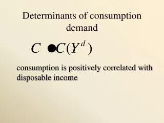
The Keynesian Theory of Consumption Keynes suggested that consumption is a positive function of income, and that high-income households consume a smaller portion of their income than low-income households. In his classic "The General Theory of Employment, Interest and Money" Keynes telling about two important things:If you find your income going up, you will spend more than you did before. But Keynes is also saying something about how much more you will spend: He predicts—based on his looking at the data and his understanding of people—thatthe rise in consumption will be less than the full rise in income. This simple observation plays a large role in helping us understand the workings of the aggregate economy.
The Keynesian Theory of Consumption The relationship between consumption and income is called the consumption function. For an individual household, the consumption function shows the level of consumption at each level of household income.
Household Consumption and Saving The aggregate consumption function shows the level of aggregate consumption at each level of aggregate income. The upward slope indicates that higher levels of income lead to higher levels of consumption spending. Y - is aggregate output (income), C - is aggregate consumption, a - is the point at which the consumption function crosses theC-axis-aconstant. b- is the slope of the line
Marginal Propensity To Consume (MPC) The slope of the consumption function (b) is called the marginal propensity to consume (MPC), or the fraction of a change in income that is consumed, or spent. marginal propensity to consume (MPC) That fraction of a change in income that is consumed, or spent.
Income, Consumption,and Saving (Y, C, and S) A household can do two, and only two, things with its income: It can consume—or it can save. Saving (S) is the part of its income that a household does not consume in a given period.Distinguished from savings, which is the current stock of accumulated saving.
Marginal Propensity To Save (MPS) The fraction of a change in income that is saved is called the marginal propensity to save (MPS). ▲S/▲Y, where ▲S - is the change in saving
MPC The marginal propensity to consume is the fraction of an increase in income that is consumed (or the fraction of a decrease in income that comes out of consumption). MPS The marginal propensity to save is the fraction of an increase in income that is saved (or the fraction of a decrease in income that comes out of saving). Because everything not consumed is saved, the MPC and the MPS must add up to 1. MPC + MPS ≡ 1
An Aggregate Consumption FunctionDerived from the Equation :
Other Determinants of Consumption The assumption that consumption depends only on income is obviously a simplification. In practice, the decisions of households on how much to consume in a given period are also affected by their wealth, by the interest rate, and by their expectations of the future. Households with higher wealth are likely to spend more, other things being equal, than households with less wealth.
Planned Investment (I) Investmentrefers to purchases by firms of new buildings andequipment and additions to inventories, all of which add to firms’ capital stock. One component of investment—inventory change—is partly determined by how much households decide to buy, which is not under the complete control of firms. planned investment (I) Those additions to capital stock and inventory that are planned by firms. actual investment The actual amount of investment that takes place; it includes items such as unplanned changes in inventories. change in inventory = production – sales
ThePlannedInvestment Function For now, we will assume that planned investment is fixed. It does not change when income changes. When a variable, such as planned investment, is assumed not to depend on the state of the economy, it is said to be an autonomous variable.
The Determination of Equilibrium Output (Income) Equilibrium occurs when there is no tendency for change. In the macroeconomic goods market, equilibrium occurs when planned aggregate expenditure is equal to aggregate output. planned aggregate expenditure (AE)The total amount the economy plans to spend in a given period. Equal to consumption plus planned investment: AE≡C + I. Y > C + I aggregate output > planned aggregate expenditure C + I > Yplanned aggregate expenditure > aggregate output
Equilibrium AggregateOutput (Income) Economy is an equilibriumwhen: Y = AEplanned aggregate expenditure AE=C + Iaggregate output Y= C + I Disequilibria: Y > C + I aggregate output > planned aggregate expenditure inventory investment is greater than plannedactual investment is greater than planned investment C + I > Yplanned aggregate expenditure > aggregate outputinventory investment is smaller than plannedactual investment is less than planned investment
(1) (2) (3) Equilibrium AggregateOutput (Income) There is only one value of Y for which this statement is true. We can find it by rearranging terms: By substituting (2) and (3) into (1) we get:
The Saving/InvestmentApproach to Equilibrium If planned investment is exactly equal to saving, then planned aggregate expenditure is exactly equal to aggregate output, andthere is equilibrium.
The Saving/InvestmentApproach to Equilibrium Because aggregate income must be saved or spent, by definition, Y≡ C + S, which is an identity. The equilibrium condition is Y = C + I, but this is not an identity because it does not hold when we are out of equilibrium. By substituting C + S for Y in the equilibrium condition, we can write: C + S = C + I Because we can subtract C from both sides of this equation, we are left with: S = I Thus, only when planned investment equals saving will there be equilibrium.
The S = I Approach to Equilibrium Aggregate output will be equal to planned aggregate expenditure only when saving equals planned investment (S = I).
Adjustment to Equilibrium The adjustment process will continue as long as output (income) is below planned aggregate expenditure. If firms react to unplanned inventory reductions by increasing output, an economy with planned spending greater than output will adjust to equilibrium, with Y higher than before. If planned spending is less than output, there will be unplanned increases in inventories. In this case, firms will respond by reducing output. As output falls, income falls, consumption falls, and so on, until equilibrium is restored, with Y lower than before.
The Multiplier multiplier The ratio of the change in the equilibrium level of output to a change in some exogenous variable. exogenous variable A variable that is assumed not to depend on the state of the economy—that is, it does not change when the economy changes.
The Multiplier At point A, the economy is in equilibrium at Y = 500. When I increases by 25, planned aggregate expenditure is initially greater than aggregate output. As output rises in response, additional consumption is generated, pushing equilibrium output up by a multiple of the initial increase in I. The new equilibrium is found at point B, where Y = 600. Equilibrium output has increased by 100 (600 - 500), or four times the amount of the increase in planned investment.
The Multiplier Equation Recall that the marginal propensity to save (MPS) is the fraction of a change in income that is saved. It is defined as the change in S (∆S) over the change in income (∆Y): Because 𝝙Smust be equal to 𝝙Ifor equilibrium to be restored, we can substitute 𝝙Ifor 𝝙Sand solve: Therefore, It follows that : , or
The Paradox of Thrift When households become concerned about the future and decide to save more, the corresponding decrease in consumption leads to a drop in spending and income. Households end up consuming less, but they have not saved any more.
The Size of the Multiplier in the Real World The multiplier is based on a very simple picture of the economy. We have assumed that planned investment is not influenced by the changes in the economy. At the same time, we ignore the role of government, financial markets and the rest of the world in the macroeconomy. For these reasons it will be a mistake to think that the national income can be increased by 100 billion by increasing planned investment spending’s by 25 billion.