Download
1 / 22
230 likes | 376 Vues
Instantaneous Monitoring of Heart Rate Variability. Outline. Abstract Introduction Methodology Results. Abstract.

E N D
Outline • Abstract • Introduction • Methodology • Results
Abstract • Most of the currently accepted approaches to compute heart rate and assess heart rate variability operate on interpolated, continuous-valued heart rate signals, thereby ignoring the underlying discrete structure of human heart beats. • To overcome this limitation, we model the stochasticstructure of heart beat intervals as a history-dependent,inverse Gaussian process and derive from it an explicitprobability density describing heart rate and heart ratevariability.
We estimate the parameters of the inverseGaussian model by local maximum likelihood and assess modelgoodness-of-fit using Q-Q plot analyses (Quantile-Quantile Normal Plots-常態分位數圖) • goodness-of-fit(適合度): 此種檢定是看我們之實際值(或觀測值)是否服從某一理論之分配。這種實際值(或觀測值)與理論值之間之配合程度之檢定問題稱之為適合度檢定。
We apply our model inan analysis ofhuman heart beat intervals from a tilt-tableexperiment.
Introduction • In the last 40 years, heart rate (HR) and heart rate variability (HRV) have been established as important quantitative indices of cardiovascular control by the autonomic nervous system, as well as effective diagnostic tools and predictors of mortality for diseases related to cardiovascular function and regulation
HR is the number of R-wave events (heart beats) perunit time on the electrocardiogram (ECG). • HRV is definedas the variation in the R-R intervals, i.e., in the timesbetween the R-wave events. • Neither HR nor HRV can beobserved directly from the ECG, but both must be estimatedfrom the sequence of R-R intervals
There are several methodological limitations to currentmethods used to estimate HRV. • In research studies, currenttime domain, frequency domain, dynamical systems, andentropy methods for HRV analysis generallyrequire several minutes or more of ECG measurements inorder to produce meaningful analyses, and these data oftenmust be collected under stationary conditions.
In addition,most of these methods must convert R-R interval data intoevenly spaced, continuous-valued measurements foranalysis by first interpolating the HR series estimatecomputed from either the local averages model or thereciprocal model • While all of these methods give importantcharacterizations of human heart beat dynamics, noneprovides a goodness-of-fit assessment to measure how wellthe R-R interval data are described by a particular model.
In response to these shortcomings, we present a new statistical framework that models the R-wave events as a discrete event defined by an inverse Gaussian parametric probability function • As such, our approach is able to avoid the need forconversion to continuous-valued signals and is also able to formally assess model goodness-of-fit through well established techniques for comparing discrete events models.
Methdology • A. Heart Rate Probability Model • In an observation interval (0,T] • 0 <U1 <U2 <...,<U5 ..., <Un ≦ T as the N successive R-wave event times detected from an ECG. • Hun is the history of the R-R intervals up to Un • θ is a set of p model parameters
The history term represents the influence of recent parasympathetic and sympathetic inputs to the SA node on the R-R interval length by modeling the mean as a linear function of the previous R-R intervals. • The Mean and Standard deviation of the R-R interval probability model in (1) are , respectively:
高斯分佈 • 早在18世紀就有數學家和天文學家開始探討這樣的一條曲線。德國天文家兼數學家高斯(Carl Friedrich Gauss,1777-1855)利用常態分佈研究天文學觀察中誤差的分佈情形,因此常態分佈又稱高斯分佈。 • 另一位著名的數學和統計學家Karl Pearson(1857-1936)將高斯分佈稱為常態分佈。
這條曲線的數學函數為 • 其中p = 3.1416,e是自然對數之底2.7183,X介在正負無限大,m是平均數,s是標準差。一旦確定平均數和標準差後,帶入公式算得f(X)。
要決定常態分佈的形狀,就必須知道平均數m和變異數s2(或者標準差s)。常態分佈取決於兩個參數(parameter):m和s2。要決定常態分佈的形狀,就必須知道平均數m和變異數s2(或者標準差s)。常態分佈取決於兩個參數(parameter):m和s2。 • 只要設定這兩個參數,就可以畫出那條常態分佈曲線。只要m或s2不同,曲線就不同。 • 這也就是為何在上述公式裡,表明 其中分號後面代表的就是決定這個函數的參數。假如變數X服從常態分佈,平均數為m,變異數為s2,則寫成:X ~ N(m, s2),其中~表示服從,N表示常態分佈。
B. Model Goodness-of-Fit • Because the R-R interval model in (1) defines an explicit discrete event model, we can use a quantile-quantile (Q-Q) analysis to evaluate model goodness-of-fit
Fig. 2. Autoregressive spectral estimation of the supine (top panel) and the tilt (bottom panel) segments of the interpolated reciprocal R-R intervals in Fig. 1A (dotted line) and our HR estimates in Fig. 1C (solid line).