Download
1 / 55
550 likes | 567 Vues
This presentation outlines the background, capabilities, and future prospects of CARMA (Combined Array for Research in Millimeter Astronomy). It discusses the science example of determining the clump mass spectrum in molecular clouds and its relation to the Initial Mass Function (IMF). It also compares CARMA with other arrays and showcases scientific examples. The presentation highlights the improved sensitivity, high dynamic range imaging, and better u,v plane sampling offered by CARMA. It concludes with a scientific example on the determination of the IMF.

E N D
CARMA(Combined Array for Research in Millimeter Astronomy)Capabilities and Future Prospects Dick Plambeck SF/ISM Seminar, 9/5/2006
outline • background • capabilities • what is CARMA good for? • science example: does the clump mass spectrum in molecular clouds determine the IMF?
Berkeley-Illinois-Maryland array 10 6.1-m diameter antennas CEDAR FLAT Caltech array 6 10.4-m antennas + UChicago SZA 8 3.5-m antennas
Cedar Flat Apr 2004 Aug 2005
panel adjustmentsurface error determined from holography before adjustment: 127 μm rms → 75% loss at 225 GHz after adjustment: 28 μm rms → 7% loss at 225 GHz
95 GHz continuum map of SS43325 Aug 2006 25 Aug 2006 rms noise 0.6 mJy/beam
basics incoming signals accepted: 3mm 80-116 GHz 1mm 220-270 GHz correlator downconverted (1-5 GHz), amplified signal sent to lab on optical fiber mostly noise from sky and receiver; source contributes < 10-3 cross-correlation spectrum
13CO 110.20 GHz 12CO 115.27 GHz LO1 112.73 GHz tuning example • LO1 tunable 85 -115 GHz, or 220 -270 GHz (1) • receive 4 GHz wide bands above (USB) and below (LSB) LO1 (2) • 8 independent spectrometers process (USB+LSB) (3) • USB and LSB signals separated in each spectrometer sky freq BIMA, OVRO correlator sections (1) no 1mm band on OVRO yet; (2) currently 1.5 GHz for BIMA 3mm receivers; (3) currently only 2.5
Cedar FlatE-array(most compact)synth beam 4.5" at 230 GHz Highway 168
BIMA antennas within collision range SZA provides even shorter spacings combine with single dish measurements from 10.4-m antennas E-array
what can we do now that we couldn’t do before? • better site should allow routine observing at 1.3 mm • much improved sensitivity (3 x collecting area of BIMA, 5 x instantaneous bandwidth) • high dynamic range imaging owing to more baselines, hence better sampling of u,v plane
225 GHz zenith opacity Tsys computed for 1.5 airmasses, Trcvr(DSB) = 45 K
sensitivity examples • 5σ detection of dust continuum from .04 Mo clump at 300 pc (5 mJy at 230 GHz) • 5σ detection of 1-0 CO emission from 2500 Mo cloud in M33 (2.5 K in 3’’ beam, ΔV = 2 km/sec)
Comparison of u,v coverage6 hr track on source at decl +10º OVRO E, 15 baselines CARMA D, 105 baselines
problems with poor u,v sampling • missing Fourier components (u,v spacings) → an infinite number of maps are consistent with the data! • how can we publish papers? sources with a few compact components are no problem • CLEAN, max entropy methods are ways of interpolating/extrapolating based on our bias about the sources (e.g., sources consist of a few compact components).
CLEANed map, point source at centerTsys = 0; no atmospheric phase noise
CLEANed map, point source at centerTsys = 0; atmospheric phase noise 150 um at 100 m; 1% contours
extended source12 x 6 arcsec FWHM, total flux 1 Jy integrated flux = 0.006 integrated flux = 0.77
scientific examplewhat determines the IMF? • physics of infall from disk to star • ‘stars determine their own mass’ • fragmentation of interstellar clouds • some (approximately fixed) percentage of a clump mass will find its way onto the star • observational test: measure the mass spectrum of prestellar clumps • want ~ a few x 103 AU resolution, ~ 5-10’’ in nearby clouds • an example: Testi and Sargent 1998, OVRO mosaic of 5’x5’ region in Serpens
Serpens mosaic Testi & Sargent 1998 99 GHz continuum 5“ resolution, about 1500 AU noise level 0.9 mJy/beam 1σ contours beginning at +/- 3σ anything > 4.5 σ (4 mJy/beam) considered real strongest sources are ~100 mJy
cumulative mass spectrum of 26 clumps not associated with IR sources dotted line is best fitting power law, dN/dM ~ M-2.1 dashed line is Salpeter IMF, dN/dM ~ M-2.35 dash-dot line is power law characteristic of larger cores, dN/dM ~ M-1.7 (Williams, Blitz, McKee 1998) → mass spectrum of protostellar dust condensations closely resembles local IMF
strongest sources are ~100 mJy anything > 4 mJy/beam is considered real → need dynamic range of 25:1 synthesized beams are particularly ugly near declination 0
comparison with BIMA mosaic Lowest contour 2.7 mJy/beam, peak ~105 mJy, beam 5" Lowest contour 8 mJy/beam, peak 256 mJy, beam ?
2 sources (300 mJy and 12 mJy), no atmospheric phase fluctuations
same model, but include atmospheric phase fluctuations of 150 um on 100-m baseline