Parallel Applications And Tools For Cloud Computing Environments
Parallel Applications And Tools For Cloud Computing Environments. SC 10 New Orleans, USA Nov 17, 2010. Azure MapReduce. AzureMapReduce. A MapRedue runtime for Microsoft Azure using Azure cloud services Azure Compute Azure BLOB storage for in/out/intermediate data storage


Parallel Applications And Tools For Cloud Computing Environments
E N D
Presentation Transcript
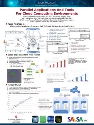
Parallel Applications And Tools For Cloud Computing Environments SC 10 New Orleans, USA Nov 17, 2010
AzureMapReduce • A MapRedue runtime for Microsoft Azure using Azure cloud services • Azure Compute • Azure BLOB storage for in/out/intermediate data storage • Azure Queues for task scheduling • Azure Table for management/monitoring data storage • Advantages of the cloud services • Distributed, highly scalable & available • Backed by industrial strength data centers and technologies • Decentralized control • Dynamically scale up/down • No Single Point of Failure
AzureMapReduce Features • Familiar MapReduce programming model • Combiner step • Fault Tolerance • Rerunning of failed and straggling tasks • Web based monitoring console • Easy testing and deployment • Customizable • Custom Input & output formats • Custom Key and value implementations • Load balanced global queue based scheduling
Advantages Fills the void of parallel programming frameworks on Microsoft Azure Well known, easy to use programming model Overcome the possible unreliability's of cloud compute nodes Designed to co-exist with eventual consistency of cloud services Allow the user to overcome the large latencies of cloud services by using coarser grained tasks Minimal management/maintanance overhead
Performance Smith WatermannPairwise Distance All-Pairs Normalized Performance CAP3 Sequence Assembly Parallel Efficiency
Pagerank with MapReduce • Efficient processing of large scale Pagerank challenges current MapReduce runtimes. • Implementations: Twister, DryadLINQ, Hadoop, MPI • Optimization strategies • Load static data in memory • Fit partition size to memory • Local merge in Reduce stage • Results Visualization with PlotViz3 • 1K 3D vertices processed with MDS • Red vertex represent “wikipedia.org”
Pagerank Optimization Strategies Implement with DryadLINQ with 50 million web pages on a 32 nodes Windows HPC cluster The coarse granularity strategy out performs fine granularity because it saves scheduling cost and network traffic Implement with Twister and Hadoop with 50 million web pages. Twister caches the partitions of web graph in memory during multiple iteration, while Hadoop needs to reload partition from disk to memory for each iteration.
Twister-BLAST A simple parallel BLAST application based on Twister MapReduce framework Runs on a single machine, a cluster, or Amazon EC2 cloud platform Adaptable to the latest BLAST tool (BLAST+ 2.2.24)
Database Management Replicated to all the nodes, in order to support BLAST binary execution Compression before replication Transported through file share script tool in Twister
Biosequence Analysis Conceptual Workflow Pairwise Clustering Cluster Indices Pairwise Alignment & Distance Calculation 3D Plot Alu Sequences Visualization Coordinates Distance Matrix Multi-Dimensional Scaling
DNA Sequencing Pipeline MapReduce Illumina/Solexa Roche/454 Life Sciences Applied Biosystems/SOLiD Pairwise clustering Blocking MDS MPI Modern Commercial Gene Sequencers Visualization Plotviz Sequence alignment Dissimilarity Matrix N(N-1)/2 values block Pairings FASTA FileN Sequences Read Alignment Internet • This chart illustrate our research of a pipeline mode to provide services on demand (Software as a Service SaaS) • User submit their jobs to the pipeline. The components are services and so is the whole pipeline.
Alu and Metagenomics Workflow “All pairs” problem Data is a collection of N sequences. Need to calculate N2dissimilarities (distances) between sequnces (all pairs). • These cannot be thought of as vectors because there are missing characters • “Multiple Sequence Alignment” (creating vectors of characters) doesn’t seem to work if N larger than O(100), where 100’s of characters long. Step 1: Can calculate N2 dissimilarities (distances) between sequences Step 2: Find families by clustering (using much better methods than Kmeans). As no vectors, use vector free O(N2) methods Step 3: Map to 3D for visualization using Multidimensional Scaling (MDS) – also O(N2) Results: N = 50,000 runs in 10 hours (the complete pipeline above) on 768 cores Discussions: • Need to address millions of sequences ….. • Currently using a mix of MapReduce and MPI • Twister will do all steps as MDS, Clustering just need MPI Broadcast/Reduce
Alu Families This visualizes results of Alu repeats from Chimpanzee and Human Genomes. Young families (green, yellow) are seen as tight clusters. This is projection of MDS dimension reduction to 3D of 35399 repeats – each with about 400 base pairs
Metagenomics This visualizes results of dimension reduction to 3D of 30000 gene sequences from an environmental sample. The many different genes are classified by clustering algorithm and visualized by MDS dimension reduction
Job Configuration and Submission Tool Microsoft HPC Cluster Submit Compute Nodes Distribute Job Cluster Head-node Sequence Aligning Pairwise Clustering Dimension Scaling PlotViz - 3D Visualization Tool Retrieve Results Write Results Biosequence Analysis Workflow Implementation
SALSA Portal Use Cases <<extend>> Create Biosequence Analysis Job
SALSA Portal Architecture
PlotViz and Dimension Reduction • http://salsahpc.org/plotviz • Currently available DirectX Windows binary • 3-6 months open source VTK/OPENGL • A tool for visualizing data points • Dimension reduction by GTM and MDS • Browse large and high-dimensional data • Use many open (value-added) data • Parallel Dimension Reduction Algorithms • GTM (Generative Topographic Mapping) • MDS (Multi-dimensional Scaling) • Interpolation extensions to GTM and MDS
PlotViz System Overview 3-D Map File SPARQL query Meta data PlotViz Light-weight client DrugBank CTD QSAR PubChem Visualization Algorithms Chem2Bio2RDF Parallel dimension reduction algorithms Aggregated public databases
Parallel Data Analysis Algorithms on Multicore Developing a suite of parallel data-analysis capabilities • Clusteringfor vectors and for points where only dissimilarities defined • Dimension Reduction for visualization and analysis (MDS, GTM) • Matrix algebraas needed • Matrix Multiplication • Equation Solving • Eigenvector/value Calculation • Extending to Global Optimization Algorithms such as Latent Dirichlet Allocation LDA • Use Deterministic Annealing for Clustering, MDS, GTM, LDA, Gaussian Mixtures …. • Extending O(N2) MDS/ dissimilarity clustering to O(NlogN)
Deterministic Annealing Clustering (DAC) • F is Free Energy • EM is well known expectation maximization method • p(x) with p(x) =1 • T is annealing temperature varied down from with final value of 1 • Determine cluster centerY(k) by EM method • K (number of clusters) starts at 1 and is incremented by algorithm N data points E(x) in D dimensions space and minimize F by EM General Deterministic Annealing Formula
Deterministic Annealing I • Gibbs Distribution at Temperature TP() = exp( - H()/T) / d exp( - H()/T) • Or P() = exp( - H()/T + F/T ) • Minimize Free EnergyF= < H- T S(P) > = d {P()H+ T P() lnP()} • Where are (a subset of) parameters to be minimized • Simulated annealing corresponds to doing these integrals by Monte Carlo • Deterministic annealing corresponds to doing integrals analytically and is naturally much faster • In each case temperature is lowered slowly – say by a factor 0.99 at each iteration
DeterministicAnnealing • Minimum evolving as temperature decreases • Movement at fixed temperature going to local minima if not initialized “correctly F({y}, T) Solve Linear Equations for each temperature Nonlinearity effects mitigated by initializing with solution at previous higher temperature Configuration {y}
Deterministic Annealing II • For some cases such as vector clustering and Gaussian Mixture Models one can do integrals by hand but usually will be impossible • So introduce Hamiltonian H0(, ) which by choice of can be made similar to H() and which has tractable integrals • P0() = exp( - H0()/T + F0/T ) approximate Gibbs • FR (P0) = < HR - T S0(P0) >|0 = < HR – H0> |0 + F0(P0) • Where <…>|0denotes d Po() • Easy to show that real Free Energy FA (PA) ≤ FR (P0) • In many problems, decreasing temperature is classic multiscale – finer resolution (T is “just” distance scale) • Same idea called variational (Bayes) inference used for Latent Dirichlet Allocation
Deterministic Annealing Clustering of Indiana Census Data Decrease temperature (distance scale) to discover more clusters Distance ScaleTemperature0.5 Redis coarse resolution with 10 clusters Blue is finer resolution with 30 clusters Clusters find cities in Indiana Distance Scale is Temperature
Implementation of DA I • Expectation step E is find minimizing FR (P0) and • Follow with M step setting = <> |0 = dPo() and if one does not anneal over all parameters and one follows with a traditional minimization of remaining parameters • In clustering, one then looks at second derivativematrixof FR (P0) wrtand as temperature is lowered this develops negative eigenvaluecorresponding to instability • This is a phase transition and one splits cluster into two and continues EM iteration • One starts with just one cluster
Rose, K., Gurewitz, E., and Fox, G. C. ``Statistical mechanics and phase transitions in clustering,'' Physical Review Letters, 65(8):945-948, August 1990. My #5 my most cited article (311)
High Performance Dimension Reduction and Visualization • Need is pervasive • Large and high dimensional data are everywhere: biology, physics, Internet, … • Visualization can help data analysis • Visualization of large datasets with high performance • Map high-dimensional data into low dimensions (2D or 3D). • Need Parallel programming for processing large data sets • Developing high performance dimension reduction algorithms: • MDS(Multi-dimensional Scaling), used earlier in DNA sequencing application • GTM(Generative Topographic Mapping) • DA-MDS(Deterministic Annealing MDS) • DA-GTM(Deterministic Annealing GTM) • Interactive visualization tool PlotViz • We are supporting drug discovery by browsing 60 million compounds in PubChem database with 166 featureseach
Dimension Reduction Algorithms • Multidimensional Scaling (MDS) [1] • Given the proximity information among points. • Optimization problem to find mapping in target dimension of the given data based on pairwise proximity information while minimize the objective function. • Objective functions: STRESS (1) or SSTRESS (2) • Only needs pairwise distances ijbetween original points (typically not Euclidean) • dij(X) is Euclidean distance between mapped (3D) points • Generative Topographic Mapping (GTM) [2] • Find optimal K-representations for the given data (in 3D), known as K-cluster problem (NP-hard) • Original algorithm use EM method for optimization • Deterministic Annealing algorithm can be used for finding a global solution • Objective functions is to maximize log-likelihood: [1] I. Borg and P. J. Groenen. Modern Multidimensional Scaling: Theory and Applications. Springer, New York, NY, U.S.A., 2005. [2] C. Bishop, M. Svens´en, and C. Williams. GTM: The generative topographic mapping. Neural computation, 10(1):215–234, 1998.
GTM vs. MDS GTM MDS (SMACOF) • MDS also soluble by viewing as nonlinear χ2 with iterative linear equation solver Purpose • Non-linear dimension reduction • Find an optimal configuration in a lower-dimension • Iterative optimization method ObjectiveFunction Maximize Log-Likelihood Minimize STRESS or SSTRESS Complexity O(KN) (K << N) O(N2) Optimization Method EM Iterative Majorization (EM-like)
MDS and GTM Map (1) PubChem data with CTD visualization by using MDS (left) and GTM (right) About 930,000 chemical compounds are visualized as a point in 3D space, annotated by the related genes in Comparative Toxicogenomics Database (CTD)
CTD data for gene-disease PubChem data with CTD visualization by using MDS (left) and GTM (right) About 930,000 chemical compounds are visualized as a point in 3D space, annotated by the related genes in Comparative Toxicogenomics Database (CTD)
Chem2Bio2RDF Chemical compounds shown in literatures, visualized by MDS (left) and GTM (right) Visualized 234,000 chemical compounds which may be related with a set of 5 genes of interest (ABCB1, CHRNB2, DRD2, ESR1, and F2) based on the dataset collected from major journal literatures which is also stored in Chem2Bio2RDF system.
Activity Cliffs GTM Visualization of bioassay activities
Solvent Screening Visualizing 215 solvents 215 solvents (colored and labeled) are embedded with 100,000 chemical compounds (colored in grey) in PubChem database
Interpolation Method • MDS and GTM are highly memory and time consuming process for large dataset such as millions of data points • MDS requires O(N2) and GTM does O(KN) (N is the number of data points and K is the number of latent variables) • Training only for sampled data and interpolating for out-of-sample set can improve performance • Interpolation is a pleasingly parallel application suitable for MapReduce and Clouds n in-sample Trained data Training N-n out-of-sample Interpolated MDS/GTM map Interpolation Total N data
Quality Comparison (O(N2) Full vs. Interpolation) MDS GTM 16 nodes • Quality comparison between Interpolated result upto 100k based on the sample data (12.5k, 25k, and 50k) and original MDS result w/ 100k. • STRESS: wij = 1 / ∑δij2 Interpolation result (blue) is getting close to the original (red) result as sample size is increasing. Time = C(250 n2 + nNI) where sample size n and NI points interpolated