A Reconfigurable Stochastic Architecture for Highly Reliable Computing
470 likes | 702 Vues
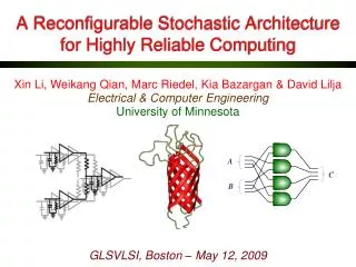
Xin Li, Weikang Qian, Marc Riedel, Kia Bazargan & David Lilja. A Reconfigurable Stochastic Architecture for Highly Reliable Computing. Electrical & Computer Engineering. University of Minnesota. GLSVLSI, Boston – May 12, 2009. Opportunities & Challenges. Topological constraints .

A Reconfigurable Stochastic Architecture for Highly Reliable Computing
E N D
Presentation Transcript
Xin Li, Weikang Qian, Marc Riedel, Kia Bazargan & David Lilja A Reconfigurable Stochastic Architecture for Highly Reliable Computing Electrical & Computer Engineering University of Minnesota GLSVLSI, Boston – May 12, 2009
Opportunities & Challenges • Topological constraints. • Inherent structural randomness. • High defect rates. Novel materials, devices, technologies: • High density of bits/logic/interconnects. Challenges for logic synthesis:
Opportunities & Challenges Strategy: • Cast synthesis in terms of arithmetic operations on real values. • Synthesize circuits that compute logical values with probabilitycorresponding to the real-valued inputs and outputs.
Probabilistic Signals deterministic deterministic random Claude E. Shannon1916 –2001 “A Mathematical Theory of Communication” Bell System Technical Journal,1948.
Probabilistic Analysis • Circuit Reliability • Probabilistic fault models. • Random test pattern generation. • Statistical Timing Power (circuit level). • Statistical Performance Measures (architectural level).
DigitalCircuit Probabilistic Analysis “There are knownknowns; and there are unknownunknowns; but today I’ll speak of the knownunknowns.” – Donald Rumsfeld, 2004 ProbabilisticInputs ProbabilisticOutputs Independent Unknown Known
DigitalCircuit Probabilistic Analysis Synthesis of Probabilistic Circuits “There are knownknowns; and there are unknownunknowns; but today I’ll speak of the knownunknowns.” – Donald Rumsfeld, 2004 ProbabilisticInputs ProbabilisticOutputs Independent Specified Unknown Unknown (for us to design) Known
Synthesis of Probabilistic Logic • Shannon and von Neumann: • “Probabilistic Logic,” • “Reliable Circuits Using Less Reliable Relays”. • K. Nepal, R. Bahar, J. Mundy, W. Patterson, and A. Zaslavsky, “Designing Logic Circuits for Probabilistic Computation in the Presence of Noise.” • L. Chakrapani, P. Korkmaz, B. Akgul, and K. Palem,“Probabilistic System-on-a-chip Architecture.”
Stochastic Logic Probability values are the input and output signals. 0.616 combinationalcircuit 0.7 0.468
Stochastic Logic + 2 0 . 6 t 0 . 4 t t - + 2 0 . 8 t 0 . 8 t 0 . 3 Probability values are the input and output signals. combinationalcircuit Functions of a probability value t.
Stochastic Logic + 2 0 . 6 t 0 . 4 t - + 2 0 . 8 t 0 . 8 t 0 . 3 = = = = Pr( X 1 ) Pr( Z 1 ) t = = Pr( Y 1 ) 0 . 3 X t 0.3 Y t Z X t Z t 0.3 Y (independently)
Stochastic Bit Streams 0,1,0,1,0 x = 2/5 X A real value x in [0, 1] is encoded as a stream of bits X.For each bit, the probability that it is one is: P(X=1) = x.
Probabilistic Bundles 0 1 x = 2/5 0 X 0 1 A real value x in [0, 1] is encoded as a stream of bits X.For each bit, the probability that it is one is: P(X=1) = x.
Stochastic Logic combinationalcircuit Probability values are the input and output signals. 4/8 5/8 3/8 4/8 3/8 8/8
Stochastic Logic combinationalcircuit Probability values are the input and output signals. 0,1,1,0,1,0,1,0,… 1,1,0,1,0,1,1,0… 0,1,1,0,1,0,0,0,… 1,0,1,0,1,0,1,0,… 1,0,0,0,1,1,0,0,… 1,1,1,1,1,1,1,1,… serial bit streams
Stochastic Logic Probability values are the input and output signals. 4/8 5/8 3/8 combinationalcircuit 4/8 3/8 8/8 parallel bit streams
Randomness A/D A/D A/D A/D A/D A/D Analog interface with fractional weighting of 1’s. combinationalcircuit parallel bit streams
Randomness LFSR Accumulator LFSR LFSR Accumulator LFSR Analog interface with fractional weighting of 1’s. combinationalcircuit parallel bit streams
Nanowire Crossbar (idealized) Randomized connections, yet nearly one-to-one.
Fault Tolerance Conventional approach: binary radix encoding. 0.111 (7/8) 0.001 (1/8) 0.010 (2/8)
Fault Tolerance Conventional approach: binary radix encoding. 0.111 (7/8) 0.101 (5/8) 0.110 (6/8) Bit flips can result in large error.
Fault Tolerance Stochastic Logic 0111111… (7/8) 01000000… (1/8) 1100000… (2/8) • Highly redundant. • Complex operations can be performed with simple logic.
Fault Tolerance Stochastic Logic 0111111… (7/8) 01000100… (2/8) 1100100… (3/8) Bit flips never result in large errors. • Highly redundant. • Complex operations can be performed with simple logic.
= c P ( C ) = c P ( C ) = P ( A ) P ( B ) = + - P ( S ) P ( A ) [ 1 P ( S )] P ( B ) = a b = + - s a ( 1 s ) b Arithmetic Operations Multiplication (Scaled) Addition 1 0
g ( t ) t combinationalcircuit Synthesizing Stochastic Logic Only polynomials… Questions: • What kinds of functions can be implemented in the probabilistic domain? • How can we synthesize the logic to implement these?
g ( t ) t combinationalcircuit Synthesizing Polynomials Only polynomials… • Implement polynomials using AND (multiplication) and MUX (scaled addition). • Must consider polynomials with coefficients less than 0 or larger than 1…
A little math… Bernstein basis polynomial of degree n
is a Bernstein coefficient A little math… Bernstein basis polynomial of degree n Bernstein polynomial of degree n
, we have Given A little math… Obtain Bernstein coefficients from power-form coefficients:
coefficients in unit interval Example: Converting a Polynomial Power-Form Polynomial Bernstein Polynomial
g ( t ) t combinationalcircuit Synthesizing Polynomials Synthesis steps: • Convert the polynomial into a Bernstein form. • Elevate it until all coefficients are in the unit interval. • Implement this with “generalized multiplexing”.
= c P ( C ) = + - P ( T ) P ( A ) [ 1 P ( T )] P ( B ) = + - t a ( 1 t ) b Bernstein polynomial Probabilistic Multiplexing
Probabilistic Multiplexing X1, …, Xn are independent Boolean random variables with Pr(Xi=1) = t, for 1 ≤ i ≤ n Z0, …, Zn are independent Boolean random variables with Pr(Zi=1)= , for 0 ≤ i ≤ n
A Reconfigurable Architecture Implement different functions by setting the coefficients:
Example Implement
Example Convert to
Non-Polynomial Functions Find a Bernstein polynomial to approximate the function: is minimized. with , such that
Non-Polynomial Functions Example: Gamma correction function. 0.45 f (t) = t Degree 6 Bernstein coefficients are: b0 = 0.0955, b1 = 0.7207, b2 = 0.3476, b3 = 0.9988, b4 = 0.7017, b5 = 0.9695, b6 = 0.9939
Deterministicv.s. StochasticImplementation of Gamma correction function with 10% noise injection. Deterministic implementation:37% pixels with errors > 20% 1% 2% 10% Conventional Implementation Stochastic Implementation: no pixels with errors > 20%! Stochastic Implementation
Comparison with Conventional Hardware Implementation of Image Processing Functions • Number of LUTs in FPGA mapping * The entire ReSC architecture, including Randomizers and De-Randomizers. ** The ReSC Unit by itself.
Comparison with Conventional Software Implementation of Image Processing Functions • Speedup (1024 cycles needed) * Software using math function from ‘Math.h’ ** Software using direct function table lookup
Comparison of Fault Tolerance for Image Processing Functions • Noise is injected in the form of a percentage of bit flips. • Percentage of Output Pixels with ErrorsGreater than 25% The stochastic implementation never produces such errors!
Comparison of Fault Tolerance for Mathematical Functions Sixth-order Maclaurin polynomial approx., 10 bits: sin(x), cos(x), tan(x), arcsin(x), arctan(x), sinh(x), cosh(x), tanh(x), arcsinh(x), exp(x), ln(x+1)
Conclusions • The hardware cost iscomparable. • Stochastic computation is much more error tolerant. • Advantage for applications where large errors are critical but small fluctuationscan be tolerated is dramatic. • (Also some pretty interesting math…) Future Directions • Apply the method at the processor level. • Apply the method at the circuit level (e.g., with PCMOS).
BiologicalProcess [computational]Synthetic Biology Quantities of Different Types ProbabilityDistribution on outcomes
X BiologicalProcess Y é ù X Z with Pr ê ú + X Y ë û [computational]Synthetic Biology fixed