Multi-Dimensional Credibility Excess Work Comp Application
Multi-Dimensional Credibility Excess Work Comp Application. Simplified Version of Least Squares Credibility in General. Loss Models Setup. An individual insured (policyholder) has n iid observations X 1 ,…,X n whose distribution is from a parameter q


Multi-Dimensional Credibility Excess Work Comp Application
E N D
Presentation Transcript
Loss Models Setup • An individual insured (policyholder) has n iid observations X1,…,Xn whose distribution is from a parameter q • q is an instance of a random variable Q with density p(q) • Define m(q) = E(Xj|Q=q) and v(q) = Var(Xj|Q=q) • m(q) is called the hypothetical mean and v(q) is the process variance • In classical statistics, m(q) is called the population mean, but Charles Hewitt, a Bayesian, considered that to be a model construct, not a truly existing entity, and so called it hypothetical, and the terminology has persisted • Let m = Em(Q), v = Ev(Q), a = Var[m(Q)] • v is the expected process variance and a is the variance of hypothetical means • Bühlmann: estimate m(q) linearly by a0+SajXj minimizing expected squared error • Answer is a0 = (1 – z)m, ai = z/n i>0 where z = n/(n+k), k = v/a • Estimates m(q) by zX* + (1 – z)m = m + z(X* – m) = EX* + z(X* – EX*) • We will generalize the left side, but derive the right side
Simplified Version • Let X* be the mean of the Xj’s • Bühlmann’s result is to estimate m(q) by zX* + (1 – z)m. • Derivation of z is much simpler if you start with that instead of a0+SajXj. • Not giving up much by this simplification because best linear estimate of the mean is the sample mean. • Assumptions imply m(q) = X* + v(q)½e = m + a½h, where e and h are independent mean 0, variance 1 deviations. • Generalize this to having two estimators X and Y of C with expected squared errors of s2 and t2, respectively, where s and t might even be random variables themselves. • Find z that minimizes E{[C – zX + (z–1)Y]2}
Finding z • Find z that minimizes E{[C – zX + (z–1)Y]2} • X = C + se, Y = C + th • Set derivative to zero • 0 = E{[C – zX + (z–1)Y][Y–X]} = E{[–zse + (z–1)th][th–se]} = E[zs2e2 + (z–1)t2h2] = zE[s2] + (z–1)E[t2] • Thusz = E(t2) / [E(s2) + E(t2)] • In the credibility model E(s2) is the expected process variance and t2 is already a constant – the variance of the hypothetical means • Also z = [1/E(s2)] / [1/E(s2) + 1/E(t2)]so the weight on X is proportional to the reciprocal of its variance, and similarly for Y • This is a standard statistical result
Workers Compensation Excess Pricing Model • Bureau excess prices traditionally based on hazard groups • Excess potential - very different across hazard groups • but also within hazard groups • Bureau methodology weights injury-type severity distributions by hazard group injury-type frequency splits • Can do that by class • Requires credibility procedure to get class distribution of losses by injury type
Severity by Injury Type, Massachusetts:Large Loss Potential Is Driven by Fatal, PT
Differences in Injury-Type Frequencies Across and Within Hazard Groups: Ratios to Temporary Total Hazard group means are very different but significant variation exists within each hazard group *95th percentile of larger classes
Correlation of Ratios to TT Across Classes Hazard Group III Use correlations to better estimate class frequencies. Major predictive of fatal and PT.
Credibility with Correlation • Denote by V, W, X, Y - class ratios to TTfor Fatal, PT, Major & Minor • Credibility Formula for Fatal for Class i: • Evi+ b(Vi– EVi) + c(Wi– EWi) + d(Xi– EXi) +e(Yi– EYi) • Here Evi= EViis the hazard group mean for Fatal:TT; b is usual z • Example credibilities for fatal for a class in HG III with 300TT claims • b = 32.6%, c = 5.0%, d = 1.3%, e = 0.2% • Major frequency - over 15 times fatal • so factor of 1.3% is in ballpark of being like 20% for fatal • Minor frequency - over 50 times fatal • so factor of 0.2% has impact of a factor of 10% for fatal (assuming differences from mean are of same magnitude as the mean) • How are these estimated?
Denote four injury types by V, W, X,andY.For the ithclass, denote the population mean ratios (i.e., the true conditional, or “hypothetical” means) as vi , wi , xi , and yi.Here these are mean ratios to TT. Credibility with Correlation
We observe each class i for each time period t. Denote byWithe class sample mean ratio for all time periods weighted byexposuresmit (TT claims),where there areNperiods ofobservation.Similarly forV, X,andY. Let midenote the sum over the time periodstof themitmis the sum over classesiof themi .Then withinVar(Wit|wi ) = sWi2/mi Notation
Assume a linear model and minimize expected squared error, where expectation is taken across all classes in the hazard group. For PT this can be expressed as minimizing:E[(a + bVi + cWi + dXi + eYi – wi )2]The coefficients sought are a, b, c, d, ande. Differentiatingwrt agives:a = – E( bVi + cWi + dXi + eYi – wi )Plugging in that foramakes the estimate ofwi = Ewi + b(Vi– EVi ) + c(Wi– EWi ) + d(Xi– EXi ) + e(Yi– EYi ) estimate of wi
We havewi = Ewi + b(Vi– EVi ) + c(Wi– EWi ) + d(Xi– EXi ) + e(Yi– EYi )Since in taking the mean across classesEwi = EWi , cis the traditional credibility factorz.The derivative ofE[(a + bVi + cWi + dXi + eYi – wi )2] wrt bgives:aEVi + E[Vi ( bVi + cWi + dXi + eYi – wi )] = 0Plugging in for athen yields:0 = E(bVi + cWi + dXi + eYi – wi )EVi + E[bVi2 + cViWi + dViXi + eViYi – Viwi]UsingCov(X,Y) = E[XY] – EXEY,this can be rearranged to give:Cov(Vi ,wi) = bVar(Vi ) + cCov(Vi ,Wi ) + dCov(Vi ,Xi ) + eCov(Vi ,Yi )Doing the same for c, d, and e will yield three more equations that look like (3), but with the variance moving over one position each time.Thus you will end up with four equations that can be written as a single matrix equation:
where C is the covariance matrix of the class by injury-type sample means Cov(Vi ,Yi ) etc. You need estimates of all covariances - like estimating the EPV and VHM But…with these you can solve this equation for b, c, d, and e to be used for PT. Repeat for the other injury types.
Comparison to NCCI Hazard GroupsSum of Squared Errors for PT/TT RatiosThree Odd Years Predicted from Three Even Years
Comparison to NCCI Hazard GroupsSum of Squared Errors for Injury Type Ratios to TTThree Odd Years Predicted from Three Even Years Conclusion: Slight improvement by this measure
Other Tests • Individual class ratios are highly variable • Grouping classes might show up the effects better • Quintiles test for a hazard group • Group the classes in the hazard group into 5 sets based on ranking predicted ratio of injury count types to TT • Look at actual vs. predicted for those sets
Sum of squared prediction errors Credibility better except for HG A Fatal and PT
Distribution of Credibility Indicated Class Means within Hazard GroupsRatio of PT / TT Counts
Distribution of Credibility Indicated Class Means within Hazard GroupsRatio of Major / TT Counts