Classification and Regression

Classification and Regression

Classification and regression • What is classification? What is regression? • Issues regarding classification and regression • Classification by decision tree induction • Bayesian Classification • Other Classification Methods • regression

What is Bayesian Classification? • Bayesian classifiers are statistical classifiers • For each new sample they provide a probability that the sample belongs to a class (for all classes)

Bayes’ Theorem: Basics • Let X be a data sample (“evidence”): class label is unknown • Let H be a hypothesis that X belongs to class C • Classification is to determine P(H|X), the probability that the hypothesis holds given the observed data sample X • P(H) (prior probability), the initial probability • E.g., X will buy computer, regardless of age, income, … • P(X): probability that sample data is observed • P(X|H) (posteriori probability), the probability of observing the sample X, given that the hypothesis holds • E.g.,Given that X will buy computer, the prob. that X is 31..40, medium income

Bayes’ Theorem • Given training dataX, posteriori probability of a hypothesis H, P(H|X), follows the Bayes theorem • Informally, this can be written as posteriori = likelihood x prior/evidence • Predicts X belongs to C2 iff the probability P(Ci|X) is the highest among all the P(Ck|X) for all the k classes • Practical difficulty: require initial knowledge of many probabilities, significant computational cost

Towards Naïve Bayesian Classifiers • Let D be a training set of tuples and their associated class labels, and each tuple is represented by an n-D attribute vector X = (x1, x2, …, xn) • Suppose there are m classes C1, C2, …, Cm. • Classification is to derive the maximum posteriori, i.e., the maximal P(Ci|X) • This can be derived from Bayes’ theorem • Since P(X) is constant for all classes, only needs to be maximized

Derivation of Naïve Bayesian Classifier • A simplified assumption: attributes are conditionally independent (i.e., no dependence relation between attributes): • This greatly reduces the computation cost: Only counts the class distribution • If Ak is categorical, P(xk|Ci) is the # of tuples in Ci having value xk for Ak divided by |Ci, D| (# of tuples of Ci in D) • If Ak is continous-valued, P(xk|Ci) is usually computed based on Gaussian distribution with a mean μ and standard deviation σ and P(xk|Ci) is

NBC: Training Dataset Class: C1:buys_computer = ‘yes’ C2:buys_computer = ‘no’ Data sample X = (age <=30, Income = medium, Student = yes Credit_rating = Fair)

NBC: An Example • P(Ci): P(buys_computer = “yes”) = 9/14 = 0.643 P(buys_computer = “no”) = 5/14= 0.357 • Compute P(X|Ci) for each class P(age = “<=30” | buys_computer = “yes”) = 2/9 = 0.222 P(age = “<= 30” | buys_computer = “no”) = 3/5 = 0.6 P(income = “medium” | buys_computer = “yes”) = 4/9 = 0.444 P(income = “medium” | buys_computer = “no”) = 2/5 = 0.4 P(student = “yes” | buys_computer = “yes) = 6/9 = 0.667 P(student = “yes” | buys_computer = “no”) = 1/5 = 0.2 P(credit_rating = “fair” | buys_computer = “yes”) = 6/9 = 0.667 P(credit_rating = “fair” | buys_computer = “no”) = 2/5 = 0.4 • X = (age <= 30 , income = medium, student = yes, credit_rating = fair) P(X|Ci) : P(X|buys_computer = “yes”) = 0.222 x 0.444 x 0.667 x 0.667 = 0.044 P(X|buys_computer = “no”) = 0.6 x 0.4 x 0.2 x 0.4 = 0.019 P(X|Ci)*P(Ci) : P(X|buys_computer = “yes”) * P(buys_computer = “yes”) = 0.028 P(X|buys_computer = “no”) * P(buys_computer = “no”) = 0.007 Therefore, X belongs to class (“buys_computer = yes”)

play tennis? Naive Bayesian Classifier Example

Naive Bayesian Classifier Example 9 5

Naive Bayesian Classifier Example • Given the training set, we compute the probabilities: • We also have the probabilities • P = 9/14 • N = 5/14

Avoiding the 0-Probability Problem • Naïve Bayesian prediction requires each conditional prob. be non-zero. Otherwise, the predicted prob. will be zero • Ex. Suppose a dataset with 1000 tuples, income=low (0), income= medium (990), and income = high (10), • Use Laplacian correction (or Laplacian estimator) • Adding 1 to each case Prob(income = low) = 1/1003 Prob(income = medium) = 991/1003 Prob(income = high) = 11/1003 • The “corrected” prob. estimates are close to their “uncorrected” counterparts

NBC: Comments • Advantages • Easy to implement • Good results obtained in most of the cases • Disadvantages • Assumption: class conditional independence, therefore loss of accuracy • Practically, dependencies exist among variables • E.g., hospitals: patients: Profile: age, family history, etc. Symptoms: fever, cough etc., Disease: lung cancer, diabetes, etc. • Dependencies among these cannot be modeled by Naïve Bayesian Classifier • How to deal with these dependencies? • Bayesian Belief Networks

Y Z P Bayesian Belief Networks • Bayesian belief network allows a subset of the variables conditionally independent • A graphical model of causal relationships • Represents dependency among the variables • Gives a specification of joint probability distribution • Nodes: random variables • Links: dependency • X and Y are the parents of Z, and Y is the parent of P • No dependency between Z and P • Has no loops or cycles X

(FH, S) (FH, ~S) (~FH, S) (~FH, ~S) LC 0.8 0.7 0.5 0.1 ~LC 0.2 0.5 0.3 0.9 Bayesian Belief Network: An Example Family History Smoker The conditional probability table (CPT) for variable LungCancer: LungCancer Emphysema CPT shows the conditional probability for each possible combination of its parents PositiveXRay Dyspnea Derivation of the probability of a particular combination of values of X, from CPT: Bayesian Belief Networks

Bayesian Belief Networks • Using Bayesian Belief Networks: • P(v1, ..., vn) = ΠP(vi/Parents(vi)) • Example: • P(LC = yes  FH = yes  S = yes) = P(FH = yes)* P(S = yes)* P(LC = yes|FH = yes  S = yes) = P(FH = yes)* P(S = yes)*0.8

Training Bayesian Networks • Several scenarios: • Given both the network structure and all variables observable: learn only the CPTs • Network structure known, some hidden variables: gradient descent (greedy hill-climbing) method • Network structure unknown, all variables observable: search through the model space to reconstruct network topology • Unknown structure, all hidden variables: No good algorithms known for this purpose

Using IF-THEN Rules for Classification • Represent the knowledge in the form of IF-THEN rules R: IF age = youth AND student = yes THEN buys_computer = yes • Rule antecedent/precondition vs. rule consequent • Assessment of a rule: coverage and accuracy • ncovers = # of tuples covered by R • ncorrect = # of tuples correctly classified by R coverage(R) = ncovers /|D| /* D: training data set */ accuracy(R) = ncorrect / ncovers • If more than one rule is triggered, need conflict resolution • Size ordering: assign the highest priority to the triggering rules that has the “toughest” requirement (i.e., with the most attribute test) • Class-based ordering: decreasing order of prevalence or misclassification cost per class • Rule-based ordering (decision list): rules are organized into one long priority list, according to some measure of rule quality or by experts

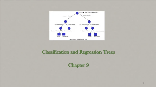
age? <=30 >40 31..40 student? credit rating? yes excellent fair no yes no yes no yes Rule Extraction from a Decision Tree • Rules are easier to understand than large trees • One rule is created for each path from the root to a leaf • Each attribute-value pair along a path forms a conjunction: the leaf holds the class prediction • Rules are mutually exclusive and exhaustive • Example: Rule extraction from our buys_computer decision-tree IF age = young AND student = no THEN buys_computer = no IF age = young AND student = yes THEN buys_computer = yes IF age = mid-age THEN buys_computer = yes IF age = old AND credit_rating = excellent THEN buys_computer = yes IF age = young AND credit_rating = fair THEN buys_computer = no

Instance-Based Methods • Instance-based learning: • Store training examples and delay the processing (“lazy evaluation”) until a new instance must be classified • Typical approaches • k-nearest neighbor approach • Instances represented as points in a Euclidean space.

. _ _ _ . _ . + . + . _ + xq . _ + The k-Nearest Neighbor Algorithm • All instances correspond to points in the n-D space. • The nearest neighbor are defined in terms of Euclidean distance. • The target function could be discrete- or real- valued. • For discrete-valued function, the k-NN returns the most common value among the k training examples nearest to xq. • Vonoroi diagram: the decision surface induced by 1-NN for a typical set of training examples.

Discussion on the k-NN Algorithm • Distance-weighted nearest neighbor algorithm • Weight the contribution of each of the k neighbors according to their distance to the query point xq • give greater weight to closer neighbors • Similarly, for real-valued target functions • Robust to noisy data by averaging k-nearest neighbors • Curse of dimensionality: distance between neighbors could be dominated by irrelevant attributes. • To overcome it, axes stretch or elimination of the least relevant attributes.

Classification and Regression