Chapter 7 Classification and Regression Trees
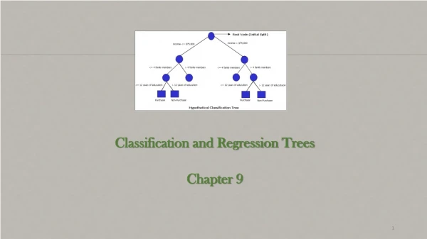
Chapter 7 Classification and Regression Trees. Introduction. What is a classification tree? The figure on the next slide describes a tree for classifying bank customers who receive a loan offer as either acceptors or non-acceptors,

Chapter 7 Classification and Regression Trees
E N D
Presentation Transcript
Introduction • What is a classification tree? • The figure on the next slide describes a tree for classifying bank customers who receive a loan offer as either acceptors or non-acceptors, • A function of information such as their income, education level, and average credit card expenditure. • Consider the tree in the example. • The square “terminal nodes" are marked with 0 or 1 corresponding to a non-acceptor (0) or acceptor (1). • The values in the circle nodes give the splitting value on a predictor. • This tree can easily be translated into a set of rules for classifying a bank customer. • For example, the middle left square node in this tree gives us the rule: • IF(Income > 92.5) AND (Education < 1.5) AND (Family · 2.5) THEN Class = 0 (non-acceptor).
Classification Trees • There are two key ideas underlying classification trees. • The first is the idea of recursive partitioning of the space of the independent variables. • The second is of pruning using validation data. • This implies the need for a third – test set. • In the following we describe recursive partitioning, and subsequent sections explain the pruning methodology.
Recursive Partitioning • Recursive partitioning divides up the p dimensional space of the x variables into non-overlapping multi-dimensional rectangles. • The X variables here are considered to be continuous, binary or ordinal. • This division is accomplished recursively (i.e., operating on the results of prior divisions). • First, one of the variables is selected, say xi, and a value of xi, say si, is chosen to split the p dimensional space into two parts: one part that contains all the points with xi <= si and the other with all the points with xi > si. • Then one of these two parts is divided in a similar manner by choosing a variable again (it could be xi or another variable) and a split value for the variable. This results in three (multi-dimensional) rectangular regions.
Recursive Partitioning • This process is continued so that we get smaller and smaller rectangular regions. • The idea is to divide the entire x-space up into rectangles such that each rectangle is as homogeneous or `pure' as possible. • By `pure' we mean containing points that belong to just one class. • (Of course, this is not always possible, as there may be points that belong to different classes but have exactly the same values for every one of the independent variables.) • Let us illustrate recursive partitioning with an example.
Riding Mowers Splitting the 24 Observations By Lot Size Value of 19 Split to reduce “impurities” within a rectangle
Measures of Impurity • There are a number of ways to measure impurity. The two most popular measures are • the Gini index and • the entropy measure • Denote the m classes of the response variable by k = 1,2,3,…,m • The Gini index and the entropy measure use pk • For a rectangle A, pk is the proportion of observations in rectangle A that belong to class k.
Gini Index Values of the Gini Index for a Two-Class Case, As a Function of the Proportion of Observations in Class 1 (p1)
Entropy Index This measure ranges between 0 (most pure, all observations belong to the same class) and log2(m) (when all m classes are equally represented). In the two-class case, the entropy measure is maximized (like the Gini index) at pk = 0.5
Evaluating the Performance of a Classification Tree • Avoiding Overfitting • Too many rectangles implies too many splits – branches • Solutions • Stopping Tree Growth: CHAID • Pruning the Tree
Stopping Tree Growth: CHAID • CHAID (Chi-Squared Automatic Interaction Detection) is a recursive partitioning method that predates classification and regression tree (CART) procedures • It uses a well-known statistical test (the chi- square test for independence) to assess whether splitting a node improves the purity by a statistically significant amount. • In particular, at each node we split on the predictor that has the strongest association with the response variable. • The strength of association is measured by the p-value of a chi-squared test of independence. • If for the best predictor the test does not show a significant improvement the split is not carried out, and the tree is terminated. • This method is more suitable for categorical predictors, but it can be adapted to continuous predictors by binning the continuous values into categorical bins.
Pruning the Tree • Grow full tree (over fit the data) • Convert decision node to leaf nodes using the CART algorithm • CART Algorithm • Uses Cost Complexity Criterion • Which is equal to the misclassification error of a tree (based on the training data) plus a penalty factor for the size of the tree. • For a tree T that has L(T) leaf nodes, the cost complexity can be written as • CC(T) = Err(T) + a*L(T) • where Err(T) is the fraction of training data observations that are misclassified by tree T and a is a “penalty factor" for tree size. • When a = 0 there is no penalty for having too many nodes in a tree and the best tree using the cost complexity criterion is the full-grown unpruned tree.
Classification Rules from Trees • Each leaf is equivalent to a classification rule. • Returning to the example on slide 3, the middle left leaf in the best pruned tree, gives us the rule: • IF(Income > 92.5) AND (Education < 1.5) AND (Family · 2.5) THEN Class = 0. • The number of rules can be reduced by removing redundancies. • IF(Income > 92.5) AND (Education > 1.5) AND (Income > 114.5) THEN Class = 1 can be simplified to • IF(Income > 114.5) AND (Education > 1.5) THEN Class = 1.
Regression Trees • The CART method can also be used for continuous response variables. • Regression trees for prediction operate in much the same fashion as classification trees. • The output variable, Y , is a continuous variable in this case, but both the principle and the procedure are the same: many splits are attempted and, for each, • We measure “impurity" in each branch of the resulting tree. • The tree procedure then selects the split that minimizes the sum of such measures.
Prediction • Predicting the value of the response Y for an observation is performed in a similar fashion to the classification case: • The predictor information is used for “dropping" down the tree until reaching a leaf node. • For instance, to predict the price of a Toyota Corolla with Age=55 and Horsepower=86, we drop it down the tree and reach the node that has the value $8842.65. • This is the price prediction for this car according to the tree. • In classification trees the value of the leaf node (which is one of the categories) is determined by the “voting" of the training data that were in that leaf. • In regression trees the value of the leaf node is determines by the average of the training data in that leaf. • In the above example, the value $8842.6 is the average of the 56 cars in the training set that fall in the category of Age > 52.5 AND Horsepower < 93.5.
Measuring Impurity • Two types of impurity measures for nodes in classification trees: • the Gini index and • the entropy-based measure. • In both cases the index is a function of the ratio between the categories of the observations in that node. • In regression trees a typical impurity measure is the sum of the squared deviations from the mean of the leaf. • This is equivalent to the squared errors, because the mean of the leaf is exactly the prediction. • In the example above, the impurity of the node with the value $8842.6 is computed by subtracting $8842.6 from the price of each of the 56 cars in the training set that fell in that leaf, then squaring these deviations, and summing them up. • The lowest impurity possible is zero, when all values in the node are equal.
Evaluating Performance • The predictive performance of regression trees can be measured in the same way that other predictive methods are evaluated, • using summary measures such as RMSE and • charts such as lift charts.
Problems • Competitive Auctions on eBay.com • Predicting Delayed Flights • Predicting Prices of Used Cars • Using Regression Trees