Chapter 7. Trees
Chapter 7. Trees. Weiqi Luo ( 骆伟祺 ) School of Software Sun Yat-Sen University Email : weiqi.luo@yahoo.com Office : A309. Chapter seven: Trees. 7.1. Trees 7.2. Labeled Trees 7.3. Tree Searching 7.4. Undirected Trees 7.5. Minimal Spanning Trees. 7.1 Trees. Tree

Chapter 7. Trees
E N D
Presentation Transcript
Chapter 7. Trees Weiqi Luo (骆伟祺) School of Software Sun Yat-Sen University Email:weiqi.luo@yahoo.com Office:A309
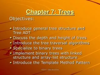
Chapter seven: Trees • 7.1. Trees • 7.2. Labeled Trees • 7.3. Tree Searching • 7.4. Undirected Trees • 7.5. Minimal Spanning Trees
7.1 Trees • Tree Let A be a set, and let T be a relation on A. We say that T is a tree if there is a vertex v0 in A with the property that #1 : there exists a unique path in T from v0 to every other vertex in A #2 : no path from v0 to v0 Usually, v0 is called the root of the tree, and T is referred to as a rooted tree (denoted by (T, v0))
7.1 Trees • Theorem 1 Let (T,v0) be a rooted tree. Then (a) There are no cycle in T (b) v0 is the only root of T (c) Each vertex in T, other than v0, has in-degree one, and v0 has in-degree zero. Proof: (a) Suppose that there is a cycle q in T, beginning and ending at vertex v. By the definition of a tree, v is not v0 and there is a path from v0 to v. The qop is a different path from v0 to v, which is a contradiction of a tree.
7.1 Trees • (b) If v0’ is another root of T, there is a path from v0 to v0’ (since v0 is a root) and a path q from v0’ to v0 (since v0’ is a root). Then qop is a cycle from v0 to v0, which is a contradiction of a tree. • (c) Let w1 be a vertex in T other than v0. There is a unique path v0, …, vk, w1, from v0 to w1 in T. Thus (vk, w1) in T, so w1 has in-degree at least one. If the in-degree of w1 is more than 1, then there must be distinct vertices w2,w3 such that (w2,w1) and (w3,w1) both in T. case #1: If w2 & w3 are not v0, there are two different paths from v0 to w1 (v0w2w1, v0w3w1, contradiction) case #2: If w2 or w3 is v0, e.g. w2=v0, there also are two different paths from v0 to w1 (v0w1, v0w3w1)
7.1 Trees • Levels, parent-offspring & siblings Level 1 vertices: the vertices of the edges beginning at v0 (level 0) . v0 Level 0 Level k vertices: the vertices of the edges beginning at those level k-1 vertices Level 1 Height of a tree: the largest level number of a tree. v1 v3 v2 Parent-offspring: for all pairs (r1, r2)in T, r1 is called the parent of r2, and r2 is called the offspring of r1 v4 Level 2 v5 v6 v7 v8 v9 Siblings: the vertices that have the same parent Leaves: the vertices that have no offsprings
7.1 Trees • Theorem 2 Let (T,v0) be a rooted tree on a set A. Then (a) T is irreflexive (b) T is asymmetric (c) If (a,b) in T and (b,c) in T, then (a,c) is not in T, for all a, b and c in A. The proof is left as an exercise.
7.1 Trees • Example 1 Let A be the set consisting of a given woman v0 and all of her female descendants. We now define the following relation T on A: If v1 and v2 are elements of A, then v1 T v2 if and only if v1 is the mother of v2. The relation T on A is a rooted three with root v0.
7.1 Trees • Example 2 Let A={v1,v2,…v10} and let T={(v2,v3), (v2,v1), (v4,v5), (v4,v6), (v5,v8), (v6,v7), (v4,v2), (v7,v9), (v7,v10)}. Show that T is a rooted tree and identify the root. v4 Root v6 v5 v2 v1 v3 v7 v8 v9 v10
7.1 Trees • n-tree If n is a positive integer, we say that a tree is an n-tree if every vertex has at most n offspring. In particular, a 2-tree is called a binary tree. • Complete n-tree If all vertices of T, other than the leaves, have exactly n offspring, we say that T is a complete n-tree. A complete 2-tree is called a completed binary tree.
T(v5) T(v2) T(v6) 7.1 Trees • Let (T,v0) be a rooted tree on the set A, and let v be a vertex of T. Let B be the set consisting of v and all its descendants, i.e., all vertices of T that can be reached by a path beginning at v. Observe that B ⊆ A. Let T(v) be the restriction of the relation T to B, that is T ∩ (B × B) . Delete all vertices that are not descendants of v and all edges that do not begin and end at any such vertex. v4 v5 v6 v2 v6 v5 v2 v1 v3 v8 v7 v1 v3 v7 v8 v9 v10 v9 v10
7.1 Trees • Theorem 3 If (T,v0) is a rooted tree and v in T, then T(v) is also a rooted tree with root v. We will say that T(v) is the subtree of T beginning at v. Proof: By the definition of T(v), there is a path from v to every other vertex in T(v). If there is a vertex w in T(v) such that there are two distinct paths q and q’ form v to w, and if p is the path in T from v0 to v, then qop and q’op would be two distinct paths in T form v0 to w (contradiction!).Thus each path from v to another vertex w in T(v) must be unique. if q is a cycle at v in T(v), then q is also a cycle in T (contradiction!). Thus q cannot exist. Therefore, T(v) is also a rooted tree with root v.
7.1 Trees • Homework Ex. 4, Ex. 10, Ex. 14, Ex. 20, Ex. 26, Ex. 27, Ex. 34
7.2 Labeled Trees • Use a tree to denote the following algebraic expression (3 - ( 2 × x ) ) + ( (x – 2 ) - ( 3 + x ) ) + 1. represent the vertices simply as dots 2. show the label of each vertex next to the dot representing that vertex - - x - + 3 Here leaves denote the numbers or variables 2 x x 2 3 x
7.2 Labeled Trees • Positional n - tree n-tree: every vertex has at most n offspring. label the offspring of a given vertex from left to right with numbers 1,2 …n 3 R L 2 R L 1 3 1 R 2 R L 3 L 3 R L 1 2 3 R R R L 2 3 1 L R L positional binary tree positional 3-tree
7.2 Labeled Trees • Huffman code trees A variable-length code widely used in lossless data compression. Base Idea: the more frequently used letters are assigned shorter strings. 0 1 Decode the string: 0101100 1 E 0: E 10: A 110: S 0: E 0 1 A 0 1 S 0 R C
7.2 Labeled Trees • Homework Ex. 8, Ex. 14, Ex. 16, Ex. 25, Ex. 27
7.3 Tree Searching • Visiting Performing appropriate tasks at a vertex will be called visiting the vertex. • Tree search The process of visiting each vertex of a tree in some specific order will be called searching the tree or performing a tree search.
7.3 Tree Searching • Algorithm PREORDER Step 1: visit v Step 2: If vL exists, then apply this algorithm to (T(vL), vL). Step 3: If vR exists, then apply this algorithm to (T(vR), vR) Recursion: Recursion is the process of repeating items in a self-similar way. Refer to http://en.wikipedia.org/wiki/Recursion
7.3 Tree Searching • Example 1 A B H C E K I 3 5 6 9 11 D F G J L 10 2 8 4 1 7 A B C D E F G H I J K L
7.3 Tree Searching • Example 2 (a – b) × (c + ( d / e) ) × - + / c a b 5 2 3 1 7 8 e d 6 4 b × — a + c / d e
7.3 Tree Searching • Prefix or Polish form ×- a b + c / d e (a=6, b=4, c=5, d=2, e=2) 1. ×- 6 4 + 5 / 2 2 2. × 2 + 5 / 2 2 replacing - 6 4 by 2 since 6-4=2 3. × 2 + 5 1 replacing / 2 2 by 1 since 2/2=1 4. × 2 6 replacing + 5 1 by 6 since 5+1=6 5. 12 replacing×2 6 by12 since 2×6=12
7.3 Tree Searching • Algorithm INORDER Step 1: Search the left subtree (T(vL), vL), if it exists; Step 2: Visit the root v; Step 3: Search the right subtree (T(vR), vR), if it exists. • Algorithm POSTORDER Step 1: Search the left subtree (T(vL), vL), if it exists; Step 2: Search the left subtree (T(vR), vR), if it exists; Step 3: Visit the root v.
7.3 Tree Searching • Traveling the tree using INORDER & POSTORDER × INORDER:a - b × c + d / e - + POSTORDER:a b – c d e / + × / c a b e d (a – b) × (c + ( d / e) )
7.3 Tree Searching • Infix notation a - b × c + d / e (a – b) × (c + ( d / e) ) or a – (b × ((c + d) / e) ) • Postfix or reverse polish a b – c d e / + × (if a=2,b=1,c=3,d=4,e=2) 1. 2 1 – 3 4 2 / + × 2. 1 3 4 2 / + × replacing 2 1 – with 1 since 2-1=1 3. 1 3 2 + × replacing 4 2 / with 2 since 4/2=2 4. 1 5 × replacing 3 2 + with 5 since 3+2=5 5. 5 replacing 1 5× with 5 since 1×5 =5
7.3 Tree Searching • Let T be any order tree and A be the set of vertices in T Define a binary positional tree B(T) on A: if v in A, the left offspring vL of v in B(T): the first offspring of v in T, if exists. the right offspring vR of v in B(T): the next sibling of v in T, if exists 1 1 2 2 3 4 3 5 4 5 6 6 7 9 10 8 11 7 12 11 13 12 13 8 9 10
7.3 Tree Searching • Homework Ex. 16, Ex. 17, Ex. 18, Ex. 24, Ex. 26, Ex. 32, Ex. 36
7.4 Undirected Trees • Undirected Tree An undirected tree is simply the symmetric closure of a tree, that is, it is the relation that results from a tree when all the edges are made bidirectional. b a b c c d e d e a d f c g f g g a b e f Note: T is the symmetric closure of T1 and T2. Thus T is a undirected tree. An undirected diagram T An ordinary tree T1 An ordinary tree T2
7.4 Undirected Trees • Simple Let R be a symmetric relation, and let p: v1,v2,…vn be a path in R. we say p is simple if no two edges of p correspond to the same undirected edge. If , in addition, v1 equals vn, we will call p a simple cycle. • Acyclic A symmetric relation R is acyclic if it contains no simple cycles. • Connected A symmetric relation R is connected if there is a path in R from any vertex to others.
7.4 Undirected Trees • Example 2 Path: a, b, c, e, d Path: f, e, d, c, d, a Path: f, e, a, d, b, a, f & d, a, b, d Path: f, e, d, c, e, f a f b e Simple Not simple, since d, c & c, d correspond to the same undirected edge. d c Simple cycles Not a simple cycle
7.4 Undirected Trees • Theorem 1 Let R be a symmetric relation on a set A. Then the following statements are equivalent. (a) R is an undirected tree (b) R is connected and acyclic
7.4 Undirected Trees • Theorem 2 Let R be a symmetric relation on a set A. Then R is an undirected tree if and only if either of the following statements is true (a) R is acyclic, and if any undirected edge is added to R, the new relation will not be acyclic; (b) R is connected, and if any undirected edge is removed from R, the new relation will not be connected.
7.4 Undirected Trees • Theorem 3 A tree with n vertices has n-1 edges Proof: Because a tree is connected, there must be at least n-1 edges to connect the n vertices. Support that there are more than n-1 edges. Then either the root has in-degree 1 or some other vertex has in-degree at least 2. But by Theorem 1, Section 7.1, this is impossible. Thus there are exactly n-1 edges. Theorem 1 (c) Each vertex in T, other than v0, has in-degree one, and v0 has in-degree zero.
7.4 Undirected Trees • Spanning Tree If R is a symmetric, connected relation on a set A, we say that a tree T on A is a spanning tree for R if T is a tree with exactly the same vertices as R and which can be obtained from R by deleting some edges of R. For instance, a a a b b b c c c e e e d d d (b) T’ (c) T’’ (a) R f f f
7.4 Undirected Trees • Undirected spanning Tree An undirected spanning tree is the symmetric closure of a spanning tree, and it is useful in some applications. a a b b c c e e d d (c) T’’ (c) Undirected Tree f f
7.4 Undirected Trees • Example 4 (d) (c) (f) (b) (a) (e) a a a a a a b b b b b b c c c c c c Theorem 2(b) & Theorem 3 suggests a simple algorithm for finding an undirected spanning tree for a symmetric relation R. e e e e e e d d d d d d f f f f f f
7.4 Undirected Trees • Merging the vertices Let R be a relation on a set A, and let a, b in A. Let A0=A-{a, b}, and A’=A0 U {a’}, where a’ is some new element not in A. Define a relation R’ on A’ as follows. Support u, v in A’, u and v are not a’. Let (a’, u) in R’ iff (a,u) in R or (b,u) in R (u, a’) in R’ iff (u,a) in R or (u,b) in R (u, v) in R’ iff (u,v) in R We say that R’ is a result of merging the vertices a and b
7.4 Undirected Trees • Example 5 v5 v5 v5 v4 v4 v4 v3 v3 v3 v0 v’0 v’’0 v6 v6 (a) R (b) Merging v1 & v0 into v’0 (c) Merging v’0 & v2 into v’’0 v1 v6 v2 v2
7.4 Undirected Trees Suppose that vertices a and b of a relation R are merged into a new vertex a’ that replaces a and b to obtain the relation R’. To determine the matrix of R’, we proceed as follows. • Step 1: Let row i represent vertex a and row j represent vertex b. Replace row i by the join of rows i and j. Note: The join of two n-tuples of 0’s and 1’s has 1 in some position exactly when either of those two n-tuples has a 1 in that position. • Step 2: Replace column i by the join of columns i and j • Step 3: Restore the main diagonal to its original values in R • Step 4: Delete row j and column j.
7.4 Undirected Trees • Example 6 v0 v’0 v1 v2 v2 v’’0 v3 v3 v3 v4 v4 v4 v5 v5 v5 v6 v6 v6 v0 v’0 v1 v2 v2 v’’0 v3 v3 v3 v4 v4 v4 v5 v5 v5 v6 v6 v6 (a) (b) (c)
7.4 Undirected Trees The Prim’s algorithm for finding a spanning tree for a symmetric, connected relation R on A={v1,v2,…,vn} • Step 1: Choose v1 of R, and arrange the matrix of R so that the first row corresponds to v1 • Step 2: Choose a vertex v2 of R such that (v1,v2) in R, merge v1 and v2 into a new vertex v’1, representing {v1,v2}, and replace v1 by v’1. compute the matrix of R’. Call the vertex v’1 a merged vertex. • Step 3: Repeat Step 1& 2 on R’ until a relation with a single vertex is obtained. At each stage, keep a record of the set of original vertices that represented by each merged vertex. • Step 4: Construct the spanning tree. At each stage, when merging vertices a & b, select an edge in R from one of the original vertices represented by a to one of the original vertices represented by b.
7.4 Undirected Trees Original & merged vertices New vertex to be merged Matrix • Example 7 d b b a’ a’’ a d c d a b a’’ a’ a c d b b c d c d d b a’ {a, c} a b d a’’ {a, c, b} c d a’’’ a’’’ {a, c, d, b} a’’’
7.4 Undirected Trees • Homework Ex. 6, Ex. 12, Ex. 14, Ex. 16, Ex. 21, Ex. 22
7.5 Minimal Spanning Trees • Weighted graph A weighted graph is a graph for which each edges is labeled with a numerical value called its weight. For instance vertices: towns edges: the distance between two connected towns B D H 6 2 3 2 3 2 5 E C A 6 4 3 5 4 G F
7.5 Minimal Spanning Trees • Example 2 B 2.6 Vertices: relay stations C 2.7 4.2 2.1 E 3.6 2.9 A I Edges: the cost for upgrading 2.4 2.2 D 4.4 2.8 3.3 2.1 3.4 1.8 2.5 J H F 3.2 5.3 1.7 G
7.5 Minimal Spanning Trees • Distance between vertices The weight of an edge (vi,vj) is sometimes referred to as the distance between vertices vi and vj. • Nearest neighbor A vertex u is nearest neighbor of vertex v if u and v are adjacent and no other vertex is joined to v by an edge of lesser weight than (u, v) (Note: may have more than one nearest neighbor)
7.5 Minimal Spanning Trees • Example 3 The nearest neighbor of A is C B D H 6 2 3 3 2 2 5 E The nearest neighbor of F is E & G C A 6 4 3 5 4 G F
7.5 Minimal Spanning Trees • The nearest neighbor of a set of vertices A vertex v is a nearest neighbor of a set vertices V={v1,v2,…,vk} in a graph if v is adjacent to some member vi of V and no other vertex adjacent to a member of V is joined by an edge of lesser weight than (v,vi). Note: This vertex v may belong to V B 2.6 C 2.7 4.2 2.1 E 3.6 2.9 A I 2.4 2.2 D 2.8 3.3 The nearest neighbor of {C,E,J} is D. 2.1 3.4 1.8 2.5 J H F 4.4 3.2 5.3 What is the nearest neighbor of {D,E,F}? 1.7 Answer: D & F G
7.5 Minimal Spanning Trees • Minimal spanning tree An undirected spanning tree in which the total weight of the edges is as small as possible, is called a minimal spanning tree. Prim’s algorithm (Section 7.4, p. 293) can easily be adapted to produce a minimal spanning tree for a weighted graph by using the greedy algorithm. Greedy algorithm makes the locally optimal choice at each stage, and hopes to find the global optimum. http://en.wikipedia.org/wiki/Greedy_algorithm
7.5 Minimal Spanning Trees Algorithm: Prim’s ALGORITHM • Step 1: Choose a vertex v1 of R. Let V={v1} and E={}; • Step 2: Choose a nearest neighbor vi of V that is adjacent to vj, vj in V, and for which the edge (vi, vj) does not form a cycle with members of E. Add vi to V and add (vi, vj) to E. • Step 3: Repeat Step 2 until |E|=n-1. Then V contains all n vertices of R, and E contains the edges of a minimal spanning tree for R.