Download
1 / 14
140 likes | 267 Vues
Population Study of Gamma Ray Bursts. S. D. Mohanty The University of Texas at Brownsville. GRB030329 Death of a massive star. GRB050709 (and three others) Evidence for binary NS mergers. Chandra. HETE error circle. (Fox et al , Nature, 2005).

E N D
Population Study of Gamma Ray Bursts S. D. Mohanty The University of Texas at Brownsville GWDAW-10, Brownsville
GRB030329Death of a massive star GWDAW-10, Brownsville
GRB050709 (and three others)Evidence for binary NS mergers Chandra HETE error circle (Fox et al, Nature, 2005) Bottom-line: The GW sources we are seeking are visible ~ once a day! GWDAW-10, Brownsville
SWIFT in operation during S5 • We should get about 100 GRB triggers • Large set of triggers and LIGO at best sensitivity = unique opportunity to conduct a deep search in the noise • Direct coincidence: detection unlikely, only UL • UL can be improved by combining GW detector data from multiple GRB triggers • Properties of the GRB population instead of any one individual member GWDAW-10, Brownsville
Maximum Likelihood approach • Data: fixed length segments from multiple IFOs for each GRB • xi for the ith GRB • Signal: Unknown signals si for the ith GRB. • Assume a maximum duration for the signals • Unknown offset from the GRB • Noise: Assume stationarity • Maximize the Likelihood over the set of offsets {i} and waveforms {si} over all the observed triggers • Mohanty, Proc. GWDAW-9, 2005 GWDAW-10, Brownsville
Detection Statistic Integration length offset x1[k] Cross-correlation (cc) x1[k] x2[k] x2[k] Segment length i (“max-cc”) Max. over offsets • Final detection statistic • = i , i=1,..,Ngrb Form of detection algorithm obtained depends on the prior knowledge used GWDAW-10, Brownsville
Analysis pipeline for S2/S3/S4 • Band pass filtering • Phase calibration • Whitening H1 Maximum over offsets from GRB arrival time Correlation coefficient with fixed integration length of 100ms H2 1 for on-source segment Several (Nsegs) from off-source data On-source pool of max-cc values Wilcoxon rank-sum test Empirical significance against Nsegs/Ngrbs off-source values LR statistic: sum of max-cc values Off-source pool Data Quality Cut GWDAW-10, Brownsville
Data Quality: test of homogeneity • Off-source cc values computed with time shifts • Split the off-source max-cc values into groups according to the time shifts • Terrestrial cross-correlation may change the distribution of cc values for different time shifts. • Distributions corresponding to shifts ti and tj • Two-sample Kolmogorov-Smirnovdistance between the distributions • Collect the sample of KS distances for all pairs of time shifts and test against known null hypothesis distribution • Results under embargo pending LSC review GWDAW-10, Brownsville
Constraining population models • The distribution of max cc depends on 9 scalar parameters • jk = h, hjk , • , = +, • j,k = detector 1, 2 • x, yjk = df x(f)y*(f)/ Sj(f) Sk(f) • Let the conditional distribution of max-cc be p(i| [jk ]i) for the ith GRB GWDAW-10, Brownsville
Constraining population models • Conditional distribution of the final statistic is P(| {[jk ]1, [jk ]2,…, [jk ]N}) • Astrophysical model: specifies the joint probability distribution of jk • Draw N times from jk , then draw once from P(| {[jk ]1, [jk ]2,…, [jk ]N}) • Repeat and build an estimate of the marginal density p() • Acceptance/rejection of astrophysical models GWDAW-10, Brownsville
Example • Euclidean universe • GRBs as standard candles in GW • Identical, stationary detectors • Only one parameter governs the distribution of max-cc : the observed matched filtering SNR • Astrophysical model: p() = 3 min3 / 4 GWDAW-10, Brownsville
Example • 100 GRBs; Delay between a GRB and GW = 1.0 sec; Maximum duration of GW signal = 100 msec • PRELIMINARY: 90% confidence belt: We should be able to exclude populations with min 1.0; Chances of ~ 5 coincident detection: 1 in 1000 GRBs. GWDAW-10, Brownsville
Future • Modify Likelihood analysis to account for extra information (Bayesian approach) • Prior information about redshift, GRB class (implies waveforms) • Use recent results from network analysis • significantly better performance than standard likelihood • Diversify the analysis to other astronomical transients • Use more than one statistic GWDAW-10, Brownsville
Probability densities • The astrophysical distribution is specified by nine scalar quantities jk = h, hjk , • , = +, • j,k = detector 1, 2 • Max-cc density depends on three scalar variables derived from jk • Linear combinations with direction dependent weights • Detector sensitivity variations taken into account at this stage • Density of final statistic (sum over max-cc) is approximately Gaussian from the central limit theorem • Confidence belt construction is computationally expensive. Faster algorithm is being implemented. GWDAW-10, Brownsville